(front)
DBSP:面向富查询语言的自动增量视图维护(DBSP: Automatic Incremental View Maintenance for Rich Query Languages)
摘要ABSTRACT
Incremental view maintenance (IVM) has long been a central problem in database theory. Many solutions have been proposed for restricted classes of database languages, such as the relational algebra, or Datalog. These techniques do not naturally generalize to richer languages. In this paper we give a general, heuristic-free solution to this problem in 3 steps: (1) we describe a simple but expressive language called DBSP for describing computations over data streams; (2) we give a new mathematical definition of IVM and a general algorithm for solving IVM for arbitrary DBSP programs, and (3) we show how to model many rich database query languages using DBSP (including the full relational algebra, queries over sets and multisets, arbitrarily nested relations, aggregation, flatmap (unnest), monotonic and non-monotonic recursion, streaming aggregation, and arbitrary compositions of all of these).
增量视图维护(incremental view maintenance, IVM)长期以来一直是数据库理论中的一个核心问题。针对受限的数据库语言类,例如关系代数或 Datalog,人们已经提出了许多解决方案。这些技术不能自然地推广到更丰富的语言。本文分 3 步给出该问题的一个通用的、不依赖启发式的解决方案:(1) 我们描述一种称为 DBSP 的简单而富有表达力的语言,用于描述数据流上的计算;(2) 我们给出 IVM 的一个新的数学定义,以及一个求解任意 DBSP 程序的 IVM 的通用算法;(3) 我们说明如何用 DBSP 为许多丰富的数据库查询语言建模(包括完整的关系代数、集合与多重集上的查询、任意嵌套的关系、聚合、展平映射(flatmap,即 unnest)、单调与非单调递归、流式聚合,以及上述这些的任意组合)。SQL 与 Datalog 都可以在 DBSP 中实现。因此,我们得到了针对用所有这些语言编写的查询的高效增量视图维护算法。
PVLDB 引用格式
Mihai Budiu, Tej Chajed, Frank McSherry, Leonid Ryzhyk, and Val Tannen. DBSP: Automatic Incremental View Maintenance for Rich Query Languages. PVLDB, 16(7): 1601-1614, 2023. doi:10.14778/3587136.3587137
PVLDB 制品可用性
Proceedings of the VLDB Endowment, Vol. 16, No. 7 ISSN 2150-8097.
doi:10.14778/3587136.3587137
1 引言1 INTRODUCTION
Incremental view maintenance (IVM) is an important and wellstudied problem in databases [25]. The IVM problem can be stated as follows: given a database 𝐷𝐵 and a view 𝑉 described by a query 𝑄 that is a function of the database, i.e. 𝑉 = 𝑄 (𝐷𝐵), maintain the contents of 𝑉 in response to changes of the database, ideally more efficiently than by simply reevaluating 𝑄 (𝐷𝐵) from scratch. We want an algorithm to evaluate 𝑄 over the changes Δ𝐷𝐵 applied to the database, since often changes are small |Δ𝐷𝐵| ≪ |𝐷𝐵|. License.
增量视图维护(incremental view maintenance, IVM)是数据库中一个重要且已被深入研究的问题 [25]。IVM 问题可以表述如下:给定数据库 $DB$ 和一个由查询 $Q$ 描述的视图 $V$,其中 $Q$ 是数据库的函数,即 $V = Q(DB)$,要求在数据库发生变化时维护 $V$ 的内容,并且最好比直接从头重新求值 $Q(DB)$ 更高效。我们希望有一个算法能在施加于数据库的变化 $\Delta DB$ 上求值 $Q$,因为变化通常很小,即 $|\Delta DB| \ll |DB|$。
For any use beyond those covered by this license, obtain permission by emailing info@vldb.org. Copyright is held by the owner/author(s). Publication rights licensed to the VLDB Endowment. doi:10.14778/3587136.3587137 This paper provides a new perspective by proposing a new definition of IVM based on a streaming model of computation. Our model is inspired by Digital Signal Processing DSP [44], applied to databases, hence the name DBSP.
本文提出一种新的视角:基于流式计算模型给出 IVM 的一个新定义。我们的模型受数字信号处理(Digital Signal Processing, DSP)[44] 的启发并应用于数据库,DBSP 由此得名。以往的 IVM 方案都建立在“定义 $Q$ 关于其输入的(偏)导数”这一概念之上,而我们的定义只要求计算流作为时间函数的导数。只要所计算的数据具有满足若干简单数学性质的“差”的概念——具体来说,构成一个阿贝尔群——流的导数就总是良定义的。(幸运的是,关系数据库可以用这种方式建模 [23, 33]。)
Whereas previous IVM solutions are based on defining a notion of a (partial) derivative of 𝑄 with respect to its inputs, our definition only requires computing derivatives of streams as functions of time. Derivatives of streams are always well-defined if the data computed on has a notion of difference that satisfies some simple mathematical properties — specifically, that it forms a commutative group. (Fortunately, relational databases can be modeled in such a way [23, 33].) DBSP has several attractive properties: (1) it is expressive.
(a) It can be used to define precisely multiple concepts: traditional queries, streaming computations, and incremental computations. (b) We have been able to express in DBSP the full relational algebra, computations over sets and bags, nested relations, aggregation, flatmap (unnest), monotonic and nonmonotonic recursion, stratified negation, while-relational programs, window queries, streaming queries, streaming aggregation, and incremental versions of all of the above. In fact, we have built a DBSP implementation of the complete SQL language (§8).
- 表达力强。(a)它可以精确地定义多个概念:传统查询、流式计算与增量计算。(b)我们已能在 DBSP 中表达完整的关系代数、集合与多重集上的计算、嵌套关系、聚合、展平映射(flatmap,即 unnest)、单调与非单调递归、分层否定、while 关系程序、窗口查询、流式查询、流式聚合,以及上述所有计算的增量版本。事实上,我们已经构建了完整的 SQL 语言的 DBSP 实现(§8)。
(2) it is simple. DBSP has only 4 operators, and it is built entirely on elementary concepts such as functions and algebraic groups.
- 简单。DBSP 只有 4 个算子,并且完全建立在函数与代数群等初等概念之上。
(3) mathematically precise. All the results in this paper have been formalized and checked using the Lean proof assistant [18].
- 数学上精确。本文所有结果都已使用 Lean 证明助手 [18] 形式化并检查过。
(4) it is modular, in the following two ways: (a) the incremental version of a complex query can be reduced recursively to incrementalizing its component subqueries. This gives a simple, syntactic, heuristic-free algorithm (Algorithm 4.6) that converts an arbitrary DBSP query plan to its incremental form. (b) Extending DBSP to support new primitive operators is easy, and they immediately benefit from the rest of the theory of incrementalization. An important consequence of modularity is that the theory can be efficiently implemented, as we briefly discuss in §8.
- 模块化,表现在以下两个方面:(a)复杂查询的增量版本可以递归地归约为对其各子查询的增量化。由此得到一个简单的、基于语法的、无需启发式的算法(算法 4.6),它能把任意 DBSP 查询计划转换为增量形式。(b)将 DBSP 扩展到支持新的原语算子很容易,而且这些算子会立即受益于增量化的其余理论。模块化的一个重要推论是:该理论可以被高效实现,我们在 §8 中简要讨论这一点。
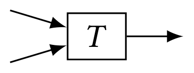
If 𝑠 ∈ S𝐴 is a stream, then 𝑠 [𝑡] ∈ 𝐴, 𝑡 ∈ N is the 𝑡-th element of 𝑠, also referred to as the value of the stream at time 𝑡. A streaming operator is a function that consumes one or more streams and produces another stream. We show streaming computations with diagrams, also called “circuits”, where boxes are computations and streams are arrows. The following diagram shows a stream operator 𝑇 : S𝐴 × S𝐵 → S𝐶 , consuming two input streams 𝑠0 and 𝑠1 and producing one output stream 𝑠: 𝑠0 𝑠1 𝑇 𝑠 We generally think of streams as sequences of “small” values, such as insertions or deletions in a database.
DBSP 的核心概念是流(stream),它用于对随时间发生的变化建模。我们用 $\mathcal{S}_A$ 表示取值为类型 $A$ 的无穷流的类型。若 $s \in \mathcal{S}_A$ 是一个流,则 $s[t] \in A$($t \in \mathbb{N}$)是 $s$ 的第 $t$ 个元素,也称为流在时刻 $t$ 的值。流算子(stream operator)是消费一个或多个流并产生另一个流的函数。我们用图——也称为“电路”(circuit)——来表示流式计算,其中方框是计算,箭头是流。下图给出一个流算子 $T : \mathcal{S}_A \times \mathcal{S}_B \to \mathcal{S}_C$,它消费两条输入流 $s_0$ 和 $s_1$,产生一条输出流 $s$:
▲ 原文(第 2 页)此处的电路图
However, we also treat the whole database as a stream of database snapshots. We model a database as a stream 𝐷𝐵 ∈ S𝑆𝐶𝐻 , where 𝑆𝐶𝐻 is the database schema. Time is not wall-clock time, but counts the transactions applied to the database. Since transactions are linearizable, they have a total order. 𝐷𝐵 [𝑡] is the snapshot of the database contents after 𝑡 transactions have been applied.
我们通常把流看作“小”值的序列,例如数据库中的插入或删除。不过,我们也把整个数据库看作一条由数据库快照构成的流。我们把数据库建模为流 $DB \in \mathcal{S}_{SCH}$,其中 $SCH$ 是数据库模式。这里的“时间”不是墙钟时间,而是对施加于数据库的事务的计数。由于事务是可线性化的,它们具有全序。$DB[t]$ 是已施加 $t$ 个事务之后数据库内容的快照。
Database transactions also form a stream Δ𝐷𝐵, this time a stream of changes, or deltas that are applied to the database. The values of this stream are defined by (Δ𝐷𝐵) [𝑡] = 𝐷𝐵 [𝑡] −𝐷𝐵 [𝑡 −1], where “−” stands for the difference between two databases, a notion that we will soon make more precise. The Δ𝐷𝐵 stream is produced from the 𝐷𝐵 stream by the stream differentiation operator D; this operator produces as its output the stream of changes from its input stream; we have thus D (𝐷𝐵) = Δ𝐷𝐵.
数据库事务也构成一条流 $\Delta DB$,这一次是施加于数据库的变化(change)或增量(delta)的流。该流的值定义为 $(\Delta DB)[t] = DB[t] - DB[t-1]$,其中“$-$”表示两个数据库之间的差,我们很快就会更精确地刻画这一概念。$\Delta DB$ 流由 $DB$ 流经流微分算子(stream differentiation operator)$\mathcal{D}$ 产生;该算子将其输入流的变化流作为输出;因此有 $\mathcal{D}(DB) = \Delta DB$。
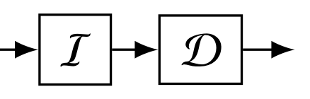
Conversely, the database snapshot at time 𝑡 is the cumulative result of applying all transactions up to 𝑡: 𝐷𝐵 [𝑡] =∑︁ 𝑖 ≤𝑡 Δ𝐷𝐵 [𝑖]. The operation I, adding up all changes, is another basic stream operator, is stream integration, the inverse of differentiation.
反过来,时刻 $t$ 的数据库快照是施加截至 $t$ 的全部事务的累积结果:$DB[t] = \sum_{i \le t} \Delta DB[i]$。把所有变化累加起来的操作 $\mathcal{I}$ 是另一个基本流算子,即流积分(stream integration),它是流微分的逆。下图给出流 $\Delta DB$ 与 $DB$ 之间的关系:
▲ 原文(第 2 页)此处的电路图
The following diagram shows the relationship between the streams Δ𝐷𝐵 and 𝐷𝐵: Δ𝐷𝐵 I 𝐷𝐵 D Δ𝐷𝐵 Suppose we are given a query 𝑄 : 𝑆𝐶𝐻 → 𝑆𝐶𝐻 defining a view 𝑉 . What is a view in a streaming model? It is also a stream! For each snapshot of the database stream we have a snapshot of the view: 𝑉 [𝑡] = 𝑄 (𝐷𝐵 [𝑡]).
假设给定一个查询 $Q : SCH \to SCH$,它定义一个视图 $V$。在流模型中视图是什么?它也是一条流!数据库流的每个快照都对应视图的一个快照:$V[t] = Q(DB[t])$。一般地,给定任意函数 $f : A \to B$,我们定义 $f$ 的流式“版本”,记作 ${\uparrow}f$(读作“$f$ 的提升”),它把 $f$ 独立地作用于输入流的每个元素。于是可以写成 $V = ({\uparrow}Q)(DB)$。
In general, given an arbitrary function 𝑓 : 𝐴 → 𝐵, we define a streaming “version” of 𝑓 , denoted by ↑𝑓 (read as “𝑓 lifted”), which applies 𝑓 to every element of the input stream independently.
有了这些基本定义,我们就可以精确地定义 IVM。增量地维护一个视图意味着什么?一个高效的维护算法需要在给定数据库变化的情况下计算视图的变化。给定查询 $Q$,本文的一个关键贡献是利用流积分与流微分定义它的增量版本 $Q^\Delta$:
$$Q^\Delta \overset{\mathrm{def}}{=} \mathcal{D} \circ {\uparrow}Q \circ \mathcal{I}.$$
We can thus write 𝑉 = (↑𝑄)(𝐷𝐵).
$$\Delta V \overset{\mathrm{def}}{=} \mathcal{D}(V) = \mathcal{D}({\uparrow}Q(\mathcal{I}(\Delta DB))),$$
Armed with these basic definitions, we can precisely define IVM.
ΔDB ──▶ [ I ] ──▶ [ ↑Q ] ──▶ [ D ] ──▶ ΔV
              DB           V
What does it mean to maintain a view incrementally? An efficient maintenance algorithm needs to compute the changes to the view given the changes to the database.
上图中,$\mathcal{I}$ 为流积分、${\uparrow}Q$ 为提升后的查询、$\mathcal{D}$ 为流微分;方框之间的中间流依次是数据库快照流 $DB$ 与视图快照流 $V$。
Given a query 𝑄, a key contribution of this paper is the definition of its incremental version 𝑄Δ, using stream integration and differentiation: 𝑄Δ def = 𝐷 ◦ ↑𝑄 ◦ 𝐼 .
查询的增量版本是一个有状态的流算子,它直接在变化上计算并产生变化。因此,查询的增量版本总是良定义的。
The incremental version of a query is thus always well-defined. The above definition shows one way to compute a query incrementally, but applying it naively produces an inefficient execution plan, since it will reconstruct the database at each step. In §3 we show how algebraic properties of the ·Δ transformation are used to optimize the implementation of 𝑄Δ. The first key property is that the incremental composition of subqueries is the composition of incremental subqueries: (𝑄1 ◦ 𝑄2)Δ = 𝑄1Δ ◦ 𝑄2Δ.
上述定义给出了增量地计算查询的一种方式,但朴素地应用它会产生低效的执行计划,因为它会在每一步重建数据库。在 §3 中我们将说明如何利用 $\cdot^\Delta$ 变换的代数性质来优化 $Q^\Delta$ 的实现。第一个关键性质是:子查询的增量组合等于各子查询增量版本的组合,即 $(Q_1 \circ Q_2)^\Delta = Q_1^\Delta \circ Q_2^\Delta$。第二个关键性质是:本质上所有基本数据库操作都有高效的增量版本。更准确地说,它们比非增量版本快 $O(|DB|/|\Delta DB|)$ 倍。
More precisely, they are faster than non-incremental versions by a factor of 𝑂 (|𝐷𝐵|/|Δ𝐷𝐵|). Armed with this general theory of incremental computation, in §4 we show how to model relational queries in DBSP. This immediately gives us a general algorithm to compute the incremental version of any relational query. These results were previously known, but they are cleanly modeled by DBSP. §5.1 shows how stratifiedmonotonic recursive Datalog programs can be implemented in DBSP, and §6 gives incremental streaming computations for recursive programs.
借助这套一般性的增量计算理论,我们在 §4 中说明如何在 DBSP 中建模关系查询。这立即给出一个计算任意关系查询增量版本的通用算法。这些结果此前已为人所知,但 DBSP 为它们提供了简洁的建模。§5.1 说明分层单调递归 Datalog 程序如何能在 DBSP 中实现,§6 给出递归程序的增量流式计算。例如,给定以自然递归方式实现的传递闭包,我们的算法能生成一个程序,在图通过添加和删除边而发生变化时高效地维护该图的传递闭包。
For example, given an implementation of transitive closure in the natural recursive way, our algorithm produces a program that efficiently maintains the transitive closure of a graph as the graph is changed by adding and deleting edges. In this paper we omit proofs, they can be found in an extensive companion technical report [12]. We have formalized this theory in the Lean proof assistant [14]; our formalization includes machinechecked proofs for all the theorems in this paper.
本文省略证明,它们可在内容详尽的配套技术报告 [12] 中找到。我们已在 Lean 证明助手 [14] 中形式化了该理论;我们的形式化包含本文所有定理的机器检查证明。
This paper makes the following contributions: (1) DBSP, a simple but expressive language for streaming computation. DBSP gives an elegant formal foundation unifying the manipulation of streaming and incremental computations.
- DBSP,一种简单而富有表达力的流式计算语言。DBSP 给出了一个优雅的形式基础,统一了对流式计算与增量计算的处理。
(2) An algorithm for incrementalizing any streaming computation expressed in DBSP.
- 一个算法,用于将 DBSP 中表达的任何流式计算增量化。
(3) An illustration of how DBSP can model various query classes, such as relational algebra, nested relations, aggregations, and stratifiedmonotonic Datalog.
- 说明 DBSP 如何建模各类查询,例如关系代数、嵌套关系、聚合,以及分层单调 Datalog。
(4) The first general and machine-checked theory of IVM.
(5) A high-performance open-source implementation of DBSP as a general-purpose streaming query engine in Rust.
- DBSP 的一个高性能开源实现,用 Rust 编写,可作为通用流式查询引擎。
2 流计算2 STREAM COMPUTATIONS
The core notion of our theory of IVM is the stream. In this section we introduce formally streams as infinite sequences of values, and define computations on streams. Stream operators (§2.1) are the basic building block of stream computations. Operators can be composed with simple rules (§2.2) into complex computational circuits.
增量视图维护(incremental view maintenance, IVM)理论的核心概念是流。本节我们形式地引入作为无限取值序列的流,并定义流上的计算。流算子(stream operator,§2.1)是流计算的基本构件。算子可以借助简单规则(§2.2)组合成复杂的计算电路。在 §2.3 中我们引入流上两个本质性的运算:积分与微分。
2.1 流与流算子2.1 Streams and stream operators
N is the set of natural numbers (from 0), B is the set of Booleans, Z is the set of integers, and R is the set of real numbers.
$\mathbb{N}$ 是自然数集(从 0 开始),$\mathbb{B}$ 是布尔值集合,$\mathbb{Z}$ 是整数集,$\mathbb{R}$ 是实数集。
Definition 2.1 (stream): Given a set 𝐴, a stream of values from 𝐴, or an 𝐴-stream, is a function N → 𝐴. We denote by S𝐴 def = {𝑠 | 𝑠 : N → 𝐴} the set of all 𝐴-streams. When 𝑠 ∈ S𝐴 and 𝑡 ∈ N we write 𝑠 [𝑡] for the 𝑡-th element of the stream 𝑠 instead of the usual 𝑠 (𝑡).
定义 2.1(流):给定集合 $A$,一个来自 $A$ 的值的流,或一个 $A$-流,是一个函数 $\mathbb{N} \to A$。我们记 $\mathcal{S}_A \overset{\mathrm{def}}{=} \{s \mid s : \mathbb{N} \to A\}$ 为所有 $A$-流的集合。
We think of the index 𝑡 ∈ N as (discrete) time and of 𝑠 [𝑡] ∈ 𝐴 as the value of the the stream 𝑠 “at time” 𝑡. For example, the stream of natural numbers 𝑖𝑑 ∈ SN given by id [𝑡] = 𝑡 is the sequence of values [ 0 1 2 3 4 · · · ].
当 $s \in \mathcal{S}_A$ 且 $t \in \mathbb{N}$ 时,我们把流 $s$ 的第 $t$ 个元素写成 $s[t]$,而不是通常的 $s(t)$。我们把下标 $t \in \mathbb{N}$ 视为(离散的)时间,把 $s[t] \in A$ 视为流 $s$ “在时刻” $t$ 的值。例如,由 $id[t] = t$ 给出的自然数流 $id \in \mathcal{S}_{\mathbb{N}}$ 就是取值序列 $[0\ 1\ 2\ 3\ 4\ \cdots]$。
定义 2.2(流算子):一个具有 $n$ 个输入的流算子是一个函数 $T : \mathcal{S}_{A_0} \times \cdots \times \mathcal{S}_{A_{n-1}} \to \mathcal{S}_B$。
Definition 2.2 (stream operator): A stream operator with 𝑛 inputs is a function 𝑇 : S𝐴0 × · · · × S𝐴𝑛−1 → S𝐵 .
一般地,我们用“算子”指流上的函数,用“函数”指“标量”值上的计算。
In general we use “operator” for functions on streams, and “function” for computations on “scalar” values. DBSP is an extension of the simply-typed lambda calculus — we will introduce its elements gradually. However, in many cases we find it more readable to use circuit diagrams to depict DBSP programs.
DBSP 是简单类型 lambda 演算的一个扩展——我们将逐步引入它的各个要素。然而,在很多情况下我们发现用电路图来描绘 DBSP 程序更易读。(电路确实隐藏了算子输入的顺序;对于非交换的算子,我们必须额外区分算子的输入。)在电路中,矩形表示一次算子应用(用算子名标注,例如 $T$),而箭头表示一个流。
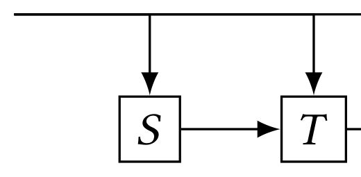
流算子的复合(函数复合)画成串联的电路。将二元算子 $T : \mathcal{S}_A \times \mathcal{S}_B \to \mathcal{S}_A$ 与一元算子 $S : \mathcal{S}_A \to \mathcal{S}_B$ 复合成计算 $\lambda s.T(T(s, S(s)), S(s)) : \mathcal{S}_A \to \mathcal{S}_A$,其电路为:
▲ 原文(第 3 页)此处的电路图
(Circuits do hide the order of the inputs of an operator; for non-commutative operators we have to distinguish the operator inputs.) In a circuit a rectangle represents an operator application (labeled with the operator name, e.g., 𝑇 ), while an arrow is a stream.
输入 $s$ 分两路:一路直接进入第一个 $T$(作为它的第一个输入),另一路先经 $S$ 得到 $S(s)$,再同时送入两个 $T$ 的第二个输入;第一个 $T$ 的输出作为第二个 $T$ 的第一个输入,第二个 $T$ 的输出即 $o$。
Stream operator composition (function composition) is shown as chained circuits. The composition of a binary operator 𝑇 : S𝐴 × S𝐵 → S𝐴 with the unary operator 𝑆 : S𝐴 → S𝐵 into the computation 𝜆𝑠.𝑇 (𝑇 (𝑠, 𝑆 (𝑠)), 𝑆 (𝑠)) : S𝐴 → S𝐴 is: 𝑠 𝑆 𝑇 𝑇 𝑆 𝑜 Definition 2.3: (lifting) Given a (scalar) function 𝑓 : 𝐴 → 𝐵, we define a stream operator ↑𝑓 : S𝐴 → S𝐵 by lifting the function 𝑓 pointwise in time: (↑𝑓 )(𝑠) def = 𝑓 ◦ 𝑠. Equivalently, ((↑𝑓 )(𝑠)) [𝑡] def = 𝑓 (𝑠 [𝑡]). This extends to functions of multiple arguments.
定义 2.3(提升):给定一个(标量)函数 $f : A \to B$,我们通过按时间逐点提升(lifting)函数 $f$ 来定义一个流算子 ${\uparrow}f : \mathcal{S}_A \to \mathcal{S}_B$:$({\uparrow}f)(s) \overset{\mathrm{def}}{=} f \circ s$。等价地,$(({\uparrow}f)(s))[t] \overset{\mathrm{def}}{=} f(s[t])$。这可以推广到具有多个参数的函数。
例如,$({\uparrow}(\lambda x.(2x)))(id) = [0\ 2\ 4\ 6\ 8\ \cdots]$。
For example, (↑(𝜆𝑥 . (2𝑥)))(𝑖𝑑) = [ 0 2 4 6 8 · · · ]. Proposition 2.4 (distributivity): Lifting distributes over function composition: ↑(𝑓 ◦ 𝑔) = (↑𝑓 ) ◦ (↑𝑔).
命题 2.4(分配律):提升对函数复合满足分配律:${\uparrow}(f \circ g) = ({\uparrow}f) \circ ({\uparrow}g)$。
We say that two DBSP programs are equivalent if they compute the same input-output function on streams. We use the symbol ≅ to indicate that two circuits are equivalent. For example, Proposition 2.4 states the following circuit equivalence: 𝑠 ↑𝑔 ↑𝑓 𝑜 ≅ 𝑠 ↑(𝑓 ◦ 𝑔) 𝑜
我们说两个 DBSP 程序是等价的,如果它们在流上计算相同的输入-输出函数。我们用符号 $\cong$ 表示两个电路等价。例如,命题 2.4 陈述了如下电路等价:
▲ 原文(第 3 页)此处的电路图
2.2 阿贝尔群上的流2.2 Streams over abelian groups
For the rest of the technical development we require the set of values 𝐴 of a stream S𝐴 to form a commutative group (𝐴, +, 0𝐴, −). The plus defines what it means to add new data, while the minus allows us to compute differences (deltas); the group structure will allow us to reorder insertions and deletions. We show later that this restriction is not a problem for using DBSP with relational data. Now we introduce some useful operators and study their properties.
在本节余下的技术展开中,我们要求流 $\mathcal{S}_A$ 的取值集合 $A$ 构成一个阿贝尔群(交换群)$(A, +, 0_A, -)$。加法定义了“加入新数据”的含义,而减法使我们能够计算差(增量);群结构将允许我们重排插入与删除。我们稍后会说明,这一限制对于把 DBSP 用于关系数据并不构成问题。现在我们引入一些有用的算子并研究它们的性质。
2.2.1 延迟与时不变性2.2.1 Delays and time-invariance.
Definition 2.5 (Delay): The delay operator1 produces an output stream by delaying its input by one step: 𝑧−1 𝐴 : S𝐴 → S𝐴: 𝑧−1 𝐴 (𝑠) [𝑡] def ={︄ 0𝐴 when 𝑡 = 0 𝑠 [𝑡 − 1] when 𝑡 ≥ 1 We often omit the type parameter 𝐴, and write just 𝑧−1.
定义 2.5(延迟):延迟算子(delay operator)[^1]通过把输入延迟一步来产生输出流:$z^{-1}_A : \mathcal{S}_A \to \mathcal{S}_A$:
$$z^{-1}_A(s)[t] \overset{\mathrm{def}}{=} \begin{cases} 0_A & \text{当 } t = 0 \\ s[t-1] & \text{当 } t \geq 1 \end{cases}$$
For example, 𝑧−1 (id) = [ 0 0 1 2 3 · · · ].
我们常常省略类型参数 $A$,只写 $z^{-1}$。例如,$z^{-1}(id) = [0\ 0\ 1\ 2\ 3\ \cdots]$。
Definition 2.6 (Time invariance): A stream operator 𝑆 : S𝐴 → S𝐵 is time-invariant (TI) if 𝑆 (𝑧−1 𝐴 (𝑠)) = 𝑧−1 𝐵 (𝑆 (𝑠)) for all 𝑠 ∈ S𝐴; in other words, if the following two circuits are equivalent: 𝑠 𝑆 𝑧−1 𝑜 ≅ 𝑠 𝑧−1 𝑆 𝑜 This definition extends naturally to operators with multiple inputs.
定义 2.6(时不变性):流算子 $S : \mathcal{S}_A \to \mathcal{S}_B$ 是时不变(time-invariant, TI)的,如果对所有 $s \in \mathcal{S}_A$ 都有 $S(z^{-1}_A(s)) = z^{-1}_B(S(s))$;换言之,如果下面两个电路等价:
▲ 原文(第 3 页)此处的电路图
The composition of TI operators of any number of inputs is TI. The delay operator 𝑧−1 is TI. DBSP only uses TI operators.
该定义自然地推广到具有多个输入的算子。任意输入个数的 TI 算子的复合仍是 TI 的。延迟算子 $z^{-1}$ 是 TI 的。DBSP 只使用时不变算子。
2.2.2 因果与严格算子2.2.2 Causal and strict operators.
Definition 2.7 (Causality): A stream operator 𝑆 : S𝐴 → S𝐵 is causal when for all 𝑠, 𝑠 ′ ∈ S𝐴, and all times 𝑡 we have: (∀𝑖 ≤ 1The name 𝑧−1 comes from the DSP literature, and is related to the z-transform [44]. 𝑡 .𝑠 [𝑖] = 𝑠 ′ [𝑖]) ⇒ 𝑆 (𝑠) [𝑡] = 𝑆 (𝑠 ′) [𝑡]. In other words, the output value at time 𝑡 can only depend on input values from times 𝑡 ′ ≤ 𝑡.
定义 2.7(因果性):流算子 $S : \mathcal{S}_A \to \mathcal{S}_B$ 是因果的(causal),当对所有 $s, s' \in \mathcal{S}_A$ 和所有时刻 $t$ 都有:
$$(\forall i \leq t.\, s[i] = s'[i]) \Rightarrow S(s)[t] = S(s')[t].$$
Operators produced by lifting are causal, and 𝑧−1 is causal. All DBSP operators are causal. The composition of causal operators of any number of inputs is causal.
换言之,时刻 $t$ 的输出值只能依赖于时刻 $t' \leq t$ 的输入值。由提升产生的算子是因果的,$z^{-1}$ 也是因果的。所有 DBSP 算子都是因果的。任意输入个数的因果算子的复合仍是因果的。
定义 2.8(严格性):流算子 $F : \mathcal{S}_A \to \mathcal{S}_B$ 是严格的(strict),如果 $\forall s, s' \in \mathcal{S}_A$、$\forall t \in \mathbb{N}$ 都有:
$$(\forall i < t.\, s[i] = s'[i]) \Rightarrow F(s)[t] = F(s')[t].$$
In other words, the 𝑡-th output of 𝐹 (𝑠) can depend only on “past” values of the input 𝑠, between 0 and 𝑡 − 1. In particular, 𝐹 (𝑠) [0] = 0𝐵 is the same for all 𝑠 ∈ S𝐴. Strict operators are causal. Lifted operators in general are not strict. 𝑧−1 is strict.
换言之,$F(s)$ 的第 $t$ 个输出只能依赖于输入 $s$ 在 0 与 $t-1$ 之间的“过去”值。特别地,$F(s)[0] = 0_B$ 对所有 $s \in \mathcal{S}_A$ 都相同。严格算子是因果的。提升算子一般而言不是严格的。$z^{-1}$ 是严格的。
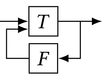
命题 2.9:对严格的 $F : \mathcal{S}_A \to \mathcal{S}_A$,方程 $\alpha = F(\alpha)$ 有唯一解 $\alpha \in \mathcal{S}_A$,记作 $\mathrm{fix}\,\alpha.F(\alpha)$。
Proposition 2.9: For a strict 𝐹 : S𝐴 → S𝐴 the equation 𝛼 = 𝐹 (𝛼) has a unique solution 𝛼 ∈ S𝐴, denoted by fix 𝛼.𝐹 (𝛼).
因此,每个从集合到自身的严格算子都有唯一的不动点。这个简单的证明依赖强归纳法,说明解 $\alpha[t]$ 只依赖于 $\alpha$ 在 $t$ 之前的值。
Thus every strict operator from a set to itself has a unique fixed point.
▲ 原文(第 3 页)此处的电路图
The simple proof relies on strong induction, showing that the solution 𝛼 [𝑡] depends only on the values of 𝛼 prior to 𝑡.
(反馈边上的 $F$ 从输出 $\alpha$ 取输入,其输出作为 $T$ 的第二个输入。)该电路是流上一个良定义的函数:
引理 2.10:若 $F : \mathcal{S}_B \to \mathcal{S}_B$ 是严格的,且 $T : \mathcal{S}_A \times \mathcal{S}_B \to \mathcal{S}_B$ 是因果的,则算子 $Q(s) = \mathrm{fix}\,\alpha.T(s, F(\alpha))$ 是良定义且因果的。此外,若 $F$ 与 $T$ 都是 TI 的,则 $Q$ 也是 TI 的。
If, moreover, 𝐹 and 𝑇 are TI then so is 𝑄. All DBSP computations are built using just lifted functions and delays. We add two more operators in §6.
所有 DBSP 计算都只用提升函数和延迟来构造。我们在 §6 中再加入两个算子。
2.3 积分与微分2.3 Integration and differentiation
Remember that we require the elements of a stream to come from an abelian group 𝐴.
记住我们要求流的元素来自阿贝尔群 $A$。流本身也构成一个阿贝尔群:
Streams themselves form an abelian group: Proposition 2.11: The structure (S𝐴, +, 0, −), obtained by lifting the + and unary − operations of 𝐴, is an abelian group. 0 is the stream with all values 0𝐴.
命题 2.11:通过提升 $A$ 的 $+$ 与一元 $-$ 运算得到的结构 $(\mathcal{S}_A, +, 0, -)$ 是一个阿贝尔群。$0$ 是所有取值均为 $0_A$ 的流。
Stream addition and negation are causal, TI operators. Definition 2.12: Given abelian groups 𝐴 and 𝐵 we call a stream operator 𝑆 : S𝐴 → S𝐵 linear if it is a group homomorphism, that is, 𝑆 (𝑎 + 𝑏) = 𝑆 (𝑎) + 𝑆 (𝑏) (and therefore 𝑆 (0) = 0 and 𝑆 (−𝑎) = −𝑆 (𝑎)).
定义 2.12:给定阿贝尔群 $A$ 与 $B$,我们称流算子 $S : \mathcal{S}_A \to \mathcal{S}_B$ 是线性的(linear),如果它是一个群同态,即 $S(a+b) = S(a) + S(b)$(从而 $S(0) = 0$ 且 $S(-a) = -S(a)$)。
Given a linear function 𝑓 : 𝐴 → 𝐵, the stream operator ↑𝑓 is linear and TI (LTI). 𝑧−1 is also LTI.
给定线性函数 $f : A \to B$,流算子 ${\uparrow}f$ 是线性且时不变的(linear and time-invariant, LTI)。$z^{-1}$ 也是 LTI 的。
Definition 2.13: (bilinear) A function of two arguments 𝑓 : 𝐴 × 𝐵 → 𝐶 with 𝐴, 𝐵, 𝐶 groups, is bilinear if it is linear separately in each argument (i.e., it distributes over addition): ∀𝑎, 𝑏, 𝑐, 𝑑.𝑓 (𝑎 + 𝑏, 𝑐) = 𝑓 (𝑎, 𝑐) + 𝑓 (𝑏, 𝑐), and 𝑓 (𝑎, 𝑐 + 𝑑) = 𝑓 (𝑎, 𝑐) + 𝑓 (𝑐, 𝑑). This definition extends to stream operators.
定义 2.13(双线性):两个参数的函数 $f : A \times B \to C$(其中 $A, B, C$ 是群)是双线性的(bilinear),如果它对每个参数分别线性(即对加法满足分配律):$\forall a, b, c, d.\,f(a+b, c) = f(a, c) + f(b, c)$,且 $f(a, c+d) = f(a, c) + f(c, d)$。
该定义推广到流算子。双线性函数 $f$ 的提升是一个双线性流算子 ${\uparrow}f$。一个例子是提升乘法:$f : \mathcal{S}_{\mathbb{N}} \times \mathcal{S}_{\mathbb{N}} \to \mathcal{S}_{\mathbb{N}}$,$f(a,b)[t] = a[t] \cdot b[t]$。
The lifting of a bilinear function 𝑓 is a bilinear stream operator ↑𝑓 .
An example is lifted multiplication: 𝑓 : SN × SN → SN, 𝑓 (𝑎, 𝑏) [𝑡] = 𝑎[𝑡] · 𝑏 [𝑡]. The “feedback loop” of a linear operator is linear: Proposition 2.14: Let 𝑆 be a unary, causal, LTI operator.
命题 2.14:设 $S$ 是一个一元、因果的 LTI 算子。则算子 $Q(s) = \mathrm{fix}\,\alpha.S(s + z^{-1}(\alpha))$ 是良定义且 LTI 的:
▲ 原文(第 3 页)此处的电路图
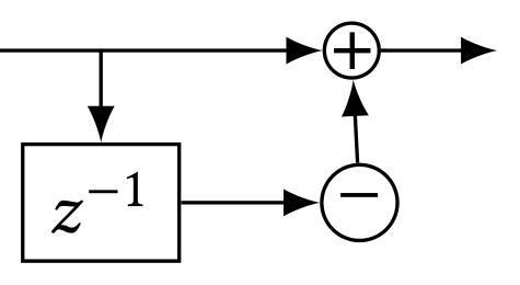
定义 2.15(微分):微分算子(differentiation operator) $\mathcal{D}_{\mathcal{S}_A} : \mathcal{S}_A \to \mathcal{S}_A$ 定义为:$\mathcal{D}(s) \overset{\mathrm{def}}{=} s - z^{-1}(s)$。
▲ 原文(第 4 页)此处的电路图
我们一般省略类型,只写 $\mathcal{D}$。若 $t > 0$,则 $\mathcal{D}(s)[t] = s[t] - s[t-1]$。例如,$\mathcal{D}(id) = [0\ 1\ 1\ 1\ 1\ \cdots]$。
The value of D (𝑠) [𝑡] = 𝑠 [𝑡] − 𝑠 [𝑡 − 1] if 𝑡 > 0. As an example, D (id) = [ 0 1 1 1 1 · · · ].
若 $s$ 是一个流,则 $\mathcal{D}(s)$ 是 $s$ 的变化流。
If 𝑠 is a stream, then D (𝑠) is the stream of changes of 𝑠. Proposition 2.16: D is causal and LTI.
命题 2.16:$\mathcal{D}$ 是因果且 LTI 的。
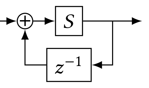
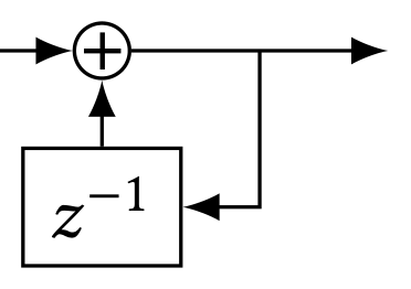
The integration operator “reconstitutes” a stream from its changes: Definition 2.17 (Integration): The integration operator IS𝐴 : S𝐴 → S𝐴 is defined by I (𝑠) def = 𝜆𝑠.fix 𝛼.
定义 2.17(积分):积分算子(integration operator) $\mathcal{I}_{\mathcal{S}_A} : \mathcal{S}_A \to \mathcal{S}_A$ 定义为 $\mathcal{I}(s) \overset{\mathrm{def}}{=} \lambda s.\,\mathrm{fix}\,\alpha.(s + z^{-1}(\alpha))$:
▲ 原文(第 4 页)此处的电路图
(𝑠 + 𝑧−1 (𝛼)): s + I (𝑠) 𝑧−1 We also generally omit the type, and write just I. This is the construction from Proposition 2.14 using the identity function for 𝑆.
我们一般也省略类型,只写 $\mathcal{I}$。这就是命题 2.14 中取 $S$ 为恒等函数的构造。
命题 2.18:$\mathcal{I}(s)$ 是施加于流 $s$ 的离散(不定)积分:$\mathcal{I}(s)[t] = \sum_{i \leq t} s[i]$。
例如,$\mathcal{I}(id) = [0\ 1\ 3\ 6\ 10\ \cdots]$。
As an example, I (id) = [ 0 1 3 6 10 · · · ]. Proposition 2.19: I is causal and LTI.
命题 2.19:$\mathcal{I}$ 是因果且 LTI 的。
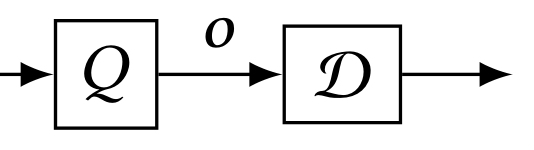
定理 2.20(互逆):积分与微分互为逆运算:$\forall s.\,\mathcal{I}(\mathcal{D}(s)) = \mathcal{D}(\mathcal{I}(s)) = s$。
▲ 原文(第 4 页)此处的电路图
Theorem 2.20 (Inversion): Integration and differentiation are inverses of each other: ∀𝑠. I (D (𝑠)) = D (I (𝑠)) = 𝑠. 𝑠 I D 𝑜 ≅ 𝑠 𝑜 ≅ 𝑠 D I 𝑜
[^1]: 名称 $z^{-1}$ 来自数字信号处理(digital signal processing, DSP)文献,与 z 变换(z-transform)[44] 有关。
3 增量视图维护3 INCREMENTAL VIEW MAINTENANCE
Here we define IVM and analyze its properties.
本节我们定义增量视图维护(incremental view maintenance, IVM)并分析其性质。
Definition 3.1: Given a unary stream operator 𝑄 : S𝐴 → S𝐵 we define the incremental version of 𝑄 as: 𝑄Δ def = D ◦ 𝑄 ◦ I.
定义 3.1:给定一元流算子 $Q : \mathcal{S}_A \to \mathcal{S}_B$,我们定义 $Q$ 的增量版本为:
$$Q^{\Delta} \overset{\text{def}}{=} \mathcal{D} \circ Q \circ \mathcal{I}. \qquad (3.1)$$
$Q^{\Delta}$ 与 $Q$ 具有相同的“类型”:$Q^{\Delta} : \mathcal{S}_A \to \mathcal{S}_B$。对于有多个输入的算子,我们通过对每个输入独立地施加 $\mathcal{I}$ 来定义其增量版本:例如,若 $T : \mathcal{S}_A \times \mathcal{S}_B \to \mathcal{S}_C$,则 $T^{\Delta}(a, b) \overset{\text{def}}{=} \mathcal{D}(T(\mathcal{I}(a), \mathcal{I}(b)))$。
▲ 原文(第 4 页)此处的电路图
(3.1) 𝑄Δ has the same “type” as 𝑄: 𝑄Δ : S𝐴 → S𝐵 .
图中 $I$ 表示积分算子 $\mathcal{I}$,$D$ 表示微分算子 $\mathcal{D}$;$s$ 与 $o$ 是流,$\Delta s$ 与 $\Delta o$ 是变化流。
For an operator with multiple inputs we define the incremental version by applying I to each input independently: e.g., if 𝑇 : S𝐴 × S𝐵 → S𝐶 then 𝑇 Δ (𝑎, 𝑏) def = D (𝑇 (I (𝑎), I (𝑏))). Δ𝑠 I 𝑄 D Δ𝑜 𝑠 𝑜 If 𝑄 (𝑠) = 𝑜 is a computation, then 𝑄Δ performs the “same” computation as 𝑄, but between streams of changes Δ𝑠 and Δ𝑜.
若 $Q(s) = o$ 是一次计算,则 $Q^{\Delta}$ 执行与 $Q$“相同”的计算,只不过是在变化流 $\Delta s$ 与 $\Delta o$ 之间进行。
Notice that our definition of incremental computation is meaningful only for streaming computations; this is in contrast to classic definitions, e.g. [25] which consider only one change.
请注意,我们对增量计算的定义只对流式计算才有意义;这与经典定义(例如 [25])不同,后者只考虑单个变化。把该定义推广到流上操作会给我们额外的能力,尤其是在处理递归查询时。
Generalizing the definition to operate on streams gives us additional power, especially when operating with recursive queries.
- 求逆(inversion):$Q \mapsto Q^{\Delta}$ 是双射;其逆为 $Q \mapsto \mathcal{I} \circ Q \circ \mathcal{D}$。
- 不变性(invariance):$+^{\Delta} = +$,$(z^{-1})^{\Delta} = z^{-1}$,$(-)^{\Delta} = -$,$\mathcal{I}^{\Delta} = \mathcal{I}$,$\mathcal{D}^{\Delta} = \mathcal{D}$。
- 推/拉(push/pull):$Q \circ \mathcal{I} = \mathcal{I} \circ Q^{\Delta}$;$\mathcal{D} \circ Q = Q^{\Delta} \circ \mathcal{D}$。
The following proposition is one of our central results: Proposition 3.2: (Properties of the incremental version): inversion: 𝑄 ↦ → 𝑄Δ is bijective; its inverse is 𝑄 ↦ → I ◦ 𝑄 ◦ D. invariance: +Δ = +, (𝑧−1)Δ = 𝑧−1, −Δ = −, IΔ = I, DΔ = D push/pull: 𝑄 ◦ I = I ◦ 𝑄Δ; D ◦ 𝑄 = 𝑄Δ ◦ D chain: (𝑄1 ◦ 𝑄2)Δ = 𝑄1Δ ◦ 𝑄2Δ (Generalizes to multiple inputs.) add: (𝑄1 + 𝑄2)Δ = 𝑄1Δ + 𝑄2Δ cycle: (𝜆𝑠.fix 𝛼.𝑇 (𝑠, 𝑧−1 (𝛼)))Δ = 𝜆𝑠.fix 𝛼.𝑇 Δ (𝑠, 𝑧−1 (𝛼)) The chain rule states that these two circuits are equivalent: 𝑖 I 𝑄1 𝑄2 D 𝑜 ≅ 𝑖 𝑄1Δ 𝑄2Δ 𝑜 In other words, to incrementalize a composite query you can incrementalize each sub-query independently.
- 链式(chain):$(Q_1 \circ Q_2)^{\Delta} = Q_1^{\Delta} \circ Q_2^{\Delta}$(该性质可推广到有多个输入的算子)。
This gives us a simple, syntax-directed, deterministic recipe for computing the incremental version of an arbitrarily complex query.
- 加法(add):$(Q_1 + Q_2)^{\Delta} = Q_1^{\Delta} + Q_2^{\Delta}$。
The cycle rule states that the following circuits are equivalent: 𝑠 I 𝑇 D 𝑜 𝑧−1 ≅ 𝑠 𝑇 Δ 𝑜 𝑧−1 In other words, the incremental version of a feedback loop around a query is just the feedback loop with the incremental query for its body.
- 循环(cycle):$(\lambda s.\ \mathrm{fix}\ \alpha.\ T(s, z^{-1}(\alpha)))^{\Delta} = \lambda s.\ \mathrm{fix}\ \alpha.\ T^{\Delta}(s, z^{-1}(\alpha))$。
链式法则(chain rule)指出如下两个电路是等价的:
▲ 原文(第 4 页)此处的电路图
换言之,要对一个复合查询做增量化,你可以分别对每个子查询做增量化。这给了我们一个简单、由语法驱动、确定性的配方(recipe),用来计算任意复杂查询的增量版本。
循环法则(cycle rule)指出如下电路是等价的:
▲ 原文(第 4 页)此处的电路图
The significance of this result will be apparent when we implement recursive queries.
图中反馈边从 $T$(或 $T^{\Delta}$)的输出引出,经延迟算子 $z^{-1}$ 后送回该算子的输入。
To execute incremental queries efficiently, we want to compute directly on streams of changes, without integrating them.
换言之,一个查询周围反馈环的增量版本,就是把环体换成该查询的增量查询之后的同一个反馈环。当我们实现递归查询时,这个结果的重要性就会显现出来。
The invariance property above shows that stream operators +, −, and 𝑧−1 are identical to their incremental versions.
为了高效地执行增量查询,我们希望直接在变化流上计算,而不对它们做积分。上面的不变性性质表明,流算子 $+$、$-$ 与 $z^{-1}$ 和它们的增量版本完全相同。下面的定理把这一点推广到线性算子与双线性算子:
The following theorems generalize this to linear and bi-linear operators: Theorem 3.3 (Linear): For an LTI operator 𝑄 we have 𝑄Δ = 𝑄.
定理 3.3(线性):对于 LTI(线性时不变,linear time-invariant)算子 $Q$,有 $Q^{\Delta} = Q$。
Theorem 3.4 (Bilinear): For a bilinear TI operator × we have (𝑎 × 𝑏)Δ = 𝑎 × 𝑏 + 𝑧−1 (I (𝑎)) × 𝑏 + 𝑎 × 𝑧−1 (I (𝑏)) = I (𝑎) × 𝑏 + 𝑎 × 𝑧−1 (I (𝑏)).
定理 3.4(双线性):对于双线性的 TI(时不变,time-invariant)算子 $\times$,有
$$(a \times b)^{\Delta} = a \times b + z^{-1}(\mathcal{I}(a)) \times b + a \times z^{-1}(\mathcal{I}(b)) = \mathcal{I}(a) \times b + a \times z^{-1}(\mathcal{I}(b)).$$
▲ 原文(第 4 页)此处的电路图
In pictures: 𝑎 I 𝑏 I × D 𝑜≅ 𝑎 𝑏 I × I 𝑧−1 𝑧−1 × × + 𝑜 ≅ 𝑎 𝑏 I I 𝑧−1 × × + 𝑜 Rewriting Theorem 3.4 using Δ𝑎 for the stream of changes to 𝑎 we get the familiar formula for incremental equi-joins: Δ(𝑎 × 𝑏) = Δ𝑎 × Δ𝑏 + 𝑎 × (Δ𝑏) + (Δ𝑎) × 𝑏; equi-joins are indeed bilinear.
把定理 3.4 用 $\Delta a$ 表示 $a$ 的变化流改写,我们就得到熟悉的增量等值连接公式:$\Delta(a \times b) = \Delta a \times \Delta b + a \times (\Delta b) + (\Delta a) \times b$;等值连接确实是双线性的。
4 关系代数的 IVM4 IVM FOR THE RELATIONAL ALGEBRA
Results in §2 and §3 apply to streams of arbitrary group values. In this section we apply these results to IVM for relational databases.
§2 与 §3 的结果适用于任意群值上的流。本节我们把它们用于关系数据库的 IVM。正如引言所述,我们的目标是高效地计算定义数据库视图的任意关系查询 $Q$ 的增量版本。
As explained in the introduction, our goal is to efficiently compute the incremental version of any relational query 𝑄 that defines a database view. However, we face a technical problem: the I and D operators were defined on abelian groups, and relational databases in general are not abelian groups, since they operate on sets. Fortunately, there is a well-known tool in the database literature which converts set operations into group operations by using Z-sets (also called z-relations [22]) to represent sets.
然而,我们面临一个技术问题:$\mathcal{I}$ 与 $\mathcal{D}$ 算子是在阿贝尔群上定义的,而关系数据库一般并不是阿贝尔群,因为它们操作的是集合。幸运的是,数据库文献中有一个著名的工具,它通过用 ℤ-集合(ℤ-set,也称为 z-关系 [22])表示集合,把集合运算转换为群运算。
We start by defining the Z-sets group, and then we review how relational queries are converted into DBSP circuits over Z-sets. This translation is efficiently incrementalizable because many basic relational queries can be expressed using LTI Z-set operators §4.2.
我们先定义 ℤ-集合群,然后回顾关系查询如何被转换为 ℤ-集合上的 DBSP 电路。这种翻译之所以能被高效地增量化,是因为许多基本关系查询都可以用 LTI 的 ℤ-集合算子来表示(见 §4.2)。
4.1 ℤ-集合作为阿贝尔群4.1 Z-sets as an abelian group
Z-sets generalize database tables: think of a Z-set as a table where each row has an associated weight, possibly negative. Given a set 𝐴, we define Z-sets over 𝐴 as functions with finite support from 𝐴 to Z. These are functions 𝑓 : 𝐴 → Z where 𝑓 (𝑥) ≠ 0 for at most a finite number of values 𝑥 ∈ 𝐴. We also write Z[𝐴] for the type of Z-sets with elements from 𝐴.
ℤ-集合推广了数据库表:可以把 ℤ-集合想成一张表,其中每一行都关联一个权重,该权重可能为负。
Values in Z[𝐴] can be thought of as key-value maps with keys in 𝐴 and values in Z, justifying the array indexing notation. If 𝑚 ∈ Z[𝐴] we write 𝑚[𝑎] instead of 𝑚(𝑎), again using an indexing notation. A particular Z-set 𝑚 ∈ Z[𝐴] can be denoted by enumerating its elements that have non-zero weights and their corresponding weights: 𝑚 = {𝑥1 ↦ → 𝑤1, . . . , 𝑥𝑛 ↦ → 𝑤𝑛 }. We call 𝑤𝑖 ∈ Z the weight of 𝑥𝑖 ∈ 𝐴.
给定一个集合 $A$,我们定义 $A$ 上的 ℤ-集合为从 $A$ 到 $\mathbb{Z}$ 的有限支撑函数。也就是函数 $f : A \to \mathbb{Z}$,其中至多对有限个 $x \in A$ 有 $f(x) \neq 0$。我们也用 $\mathbb{Z}[A]$ 表示元素取自 $A$ 的 ℤ-集合的类型。$\mathbb{Z}[A]$ 中的值可以被看作键取自 $A$、值取自 $\mathbb{Z}$ 的键值映射,这也正是使用数组下标记号的理由。若 $m \in \mathbb{Z}[A]$,我们写 $m[a]$ 而不写 $m(a)$,同样是为了沿用下标记号。
Consider a concrete Z-set 𝑅 ∈ Z[string], defined by 𝑅 = {joe ↦ → 1, anne ↦ → −1}. 𝑅 has two elements in its domain, joe with weight 1 (so 𝑅 [joe] = 1), and anne with weight −1. We say joe ∈ 𝑅 and anne ∈ 𝑅. Since Z is an abelian ring, Z[𝐴] is also an abelian ring (and thus a group). This group (Z[𝐴], +Z[𝐴], 0Z[𝐴], −Z𝐴) has addition and subtraction defined pointwise: (𝑓 +Z[𝐴] 𝑔)(𝑥) = 𝑓 (𝑥)+𝑔(𝑥).∀𝑥 ∈ 𝐴.
一个具体的 ℤ-集合 $m \in \mathbb{Z}[A]$ 可以通过枚举其权重非零的元素及相应的权重来表示:$m = \{x_1 \mapsto w_1, \ldots, x_n \mapsto w_n\}$。我们称 $w_i \in \mathbb{Z}$ 为 $x_i \in A$ 的权重。权重可以为负。当且仅当 $m[x] \neq 0$ 时,我们写 $x \in m$。我们还写 $w \cdot x$ 来表示 $\{x \mapsto w\}$。
考虑一个具体的 ℤ-集合 $R \in \mathbb{Z}[\text{string}]$,它定义为 $R = \{\text{joe} \mapsto 1, \text{anne} \mapsto -1\}$。$R$ 的定义域中有两个元素:权重为 1 的 joe(因此 $R[\text{joe}] = 1$)和权重为 $-1$ 的 anne。我们说 $\text{joe} \in R$ 且 $\text{anne} \in R$。
由于 $\mathbb{Z}$ 是阿贝尔环,$\mathbb{Z}[A]$ 也是阿贝尔环(从而是群)。这个群 $(\mathbb{Z}[A], +_{\mathbb{Z}[A]}, 0_{\mathbb{Z}[A]}, -_{\mathbb{Z}[A]})$ 的加法与减法都是逐点定义的:$(f +_{\mathbb{Z}[A]} g)(x) = f(x) + g(x), \forall x \in A$。$\mathbb{Z}[A]$ 的 $0$ 元素是函数 $0_{\mathbb{Z}[A]}$,其定义为 $0_{\mathbb{Z}[A]}(x) = 0, \forall x \in A$。例如,$R + R = \{\text{joe} \mapsto 2, \text{anne} \mapsto -2\}$。由于 ℤ-集合构成群,§2 的所有结果都适用于 ℤ-集合上的流。
Z-sets generalize sets and bags. A set with elements from 𝐴 can be represented as a Z-set by associating a weight of 1 with each element. Bags are Z-sets where all weights are positive.
ℤ-集合推广了集合与多重集。元素取自 $A$ 的集合可以这样表示为 ℤ-集合:给每个元素关联权重 1。多重集是所有权重都为正的 ℤ-集合。关键在于,ℤ-集合还能表示对集合与多重集的任意变化。变化中的负权重表示被“删除”的元素。
Crucially, Zsets can also represent arbitrary changes to sets and bags. Negative weights in a change represent elements that are being “removed”. Definition 4.1: We say that a Z-set represents a set if the weight of every element is one. We define a function to check this property isset : Z[𝐴] → B given by: isset(𝑚) def ={︃ true if 𝑚[𝑥] = 1, ∀𝑥 ∈ 𝑚 false otherwise For our example isset(𝑅) = false, since 𝑅 [anne] = −1.
定义 4.1:若一个 ℤ-集合中每个元素的权重都为 1,则称该 ℤ-集合表示一个集合。我们定义一个函数来检查这一性质,$\mathrm{isset} : \mathbb{Z}[A] \to \mathbb{B}$,它由下式给出:
$$\mathrm{isset}(m) \overset{\text{def}}{=} \begin{cases} \text{true} & \text{若 } m[x] = 1, \forall x \in m \\ \text{false} & \text{其他情况} \end{cases}$$
对我们的例子 $\mathrm{isset}(R) = \text{false}$,因为 $R[\text{anne}] = -1$。
Definition 4.2: We say that a Z-set is positive (or a bag) if the weight of every element is positive. We define a function to check this property ispositive : Z[𝐴] → B. given by ispositive(𝑚) def ={︃ true if 𝑚[𝑥] ≥ 0, ∀𝑥 ∈ 𝐴 false otherwise We have ∀𝑚 ∈ Z[𝐴].isset(𝑚) ⇒ ispositive(𝑚). ispositive(𝑅) = false, since 𝑅 [anne] = −1. We write 𝑚 ≥ 0 when 𝑚 is positive. For positive 𝑚, 𝑛 ∈ Z[𝐴] we write 𝑚 ≥ 𝑛 for iff 𝑚 − 𝑛 ≥ 0. ≥ is a partial order.
定义 4.2:若一个 ℤ-集合中每个元素的权重都为正,则称该 ℤ-集合是正的(或一个多重集)。我们定义一个函数来检查这一性质,$\mathrm{ispositive} : \mathbb{Z}[A] \to \mathbb{B}$,它由下式给出:
$$\mathrm{ispositive}(m) \overset{\text{def}}{=} \begin{cases} \text{true} & \text{若 } m[x] \geq 0, \forall x \in A \\ \text{false} & \text{其他情况} \end{cases}$$
我们有 $\forall m \in \mathbb{Z}[A].\ \mathrm{isset}(m) \Rightarrow \mathrm{ispositive}(m)$。$\mathrm{ispositive}(R) = \text{false}$,因为 $R[\text{anne}] = -1$。
We call a function 𝑓 : Z[𝐴] → Z[𝐵] positive if it maps positive values to positive values: ∀𝑥 ∈ Z[𝐴], 𝑥 ≥ 0Z[𝐴] ⇒ 𝑓 (𝑥) ≥ 0Z[𝐵 ] . We use the same notation for functions: ispositive(𝑓 ).
当 $m$ 为正时我们写 $m \geq 0$。对于正的 $m, n \in \mathbb{Z}[A]$,当且仅当 $m - n \geq 0$ 时我们写 $m \geq n$。$\geq$ 是一个偏序。
我们称函数 $f : \mathbb{Z}[A] \to \mathbb{Z}[B]$ 是正的,如果它把正的值映射为正的值:$\forall x \in \mathbb{Z}[A],\ x \geq 0_{\mathbb{Z}[A]} \Rightarrow f(x) \geq 0_{\mathbb{Z}[B]}$。我们对函数沿用同样的记号:$\mathrm{ispositive}(f)$。
定义 4.3(distinct):函数 $\mathrm{distinct} : \mathbb{Z}[A] \to \mathbb{Z}[A]$ 把一个 ℤ-集合“转换”为集合:
$$\mathrm{distinct}(m)[x] \overset{\text{def}}{=} \begin{cases} 1 & \text{若 } m[x] > 0 \\ 0 & \text{其他情况} \end{cases}$$
While very simple, this definition of distinct has been carefully chosen to enable us to implement the relational (set) operators using Z-sets operators. Generalizing circuit diagrams. From now on we will use circuits to compute both on scalars (Z-sets in our case) and streams of Z-sets.
注意 $\mathrm{distinct}$ 从多重集中“删除”重复项,它也会消去权重为负的元素。$\mathrm{distinct}(R) = \{\text{joe} \mapsto 1\}$。这个 $\mathrm{distinct}$ 的定义虽然非常简单,却是经过仔细选择的,为的是使我们能够用 ℤ-集合算子来实现关系(集合)算子。
We use the same graphical representation for functions on streams or scalars: boxes with input and output arrows. For scalar functions the “values” of the arrows are scalars instead of streams; otherwise the interpretation of boxes as function application is unchanged. We will thus use circuits to depict relational query plans.
推广电路图。 从现在起,我们将用电路来对纯量(在我们的情形中是 ℤ-集合)以及 ℤ-集合的流进行计算。对于流上的函数或纯量上的函数,我们使用相同的图形表示:带输入箭头与输出箭头的方框。对于纯量函数,箭头上的“值”是纯量而不是流;除此之外,把方框解释为函数应用这一点不变。因此,我们将用电路来刻画关系查询计划。
4.2 实现关系算子4.2 Implementing relational operators
The fact that relational algebra can be implemented by computations on Z-sets has been shown before, e.g. [23]. The translation of the relational operators to DBSP is shown in Table 1. The first row of the table shows that a composite query is translated recursively.
关系代数可以由 ℤ-集合上的计算来实现,这一点此前已有工作表明,例如 [23]。关系算子到 DBSP 的翻译如表 1 所示。表的第一行表明,复合查询是递归地翻译的。这给了我们一个把任意关系查询计划翻译成 DBSP 电路的配方。
This gives us a recipe for translating an arbitrary relational query plan into a DBSP circuit. The translation is fairly straightforward, but many operators require the application of a distinct to produce sets. For example, 𝑎 ∪ 𝑏 = distinct (𝑎 + 𝑏), 𝑎 \ 𝑏 = distinct (𝑎 − 𝑏), (𝑎 × 𝑏)((𝑥, 𝑦)) = 𝑎[𝑥] ×𝑏 [𝑦]. Notice that the use of the distinct operator allows DBSP to model the full relational algebra, including set difference (and not just the positive fragment).
这一翻译相当直截了当,但许多算子都需要施加一个 $\mathrm{distinct}$ 才能产生集合。例如,$a \cup b = \mathrm{distinct}(a + b)$,$a \setminus b = \mathrm{distinct}(a - b)$,$(a \times b)((x, y)) = a[x] \times b[y]$。注意,正是 $\mathrm{distinct}$ 算子的使用使 DBSP 能够建模完整的关系代数,包括集合差(而不只是正片段)。
Prior work (e.g., Proposition 6.13 in [22]) has shown how some invocations of distinct can be eliminated from query plans without changing the query semantics; we will see that incremental versions of distinct operators incur significant space costs. Proposition 4.4: Let 𝑄 be one of the following Z-sets operators: filtering 𝜎, join ⊲⊳, or Cartesian product ×. Then we have ∀𝑖 ∈ Z[𝐼 ], ispositive(𝑖) ⇒ 𝑄 (distinct (𝑖)) = distinct (𝑄 (𝑖)).
已有工作(例如 [22] 中的命题 6.13)表明,在不改变查询语义的前提下,可以消去查询计划中某些 $\mathrm{distinct}$ 的调用;我们将会看到,$\mathrm{distinct}$ 算子的增量版本会带来显著的空间开销。
命题 4.4:设 $Q$ 是下列 ℤ-集合算子之一:过滤 $\sigma$、连接 $\bowtie$ 或笛卡尔积 $\times$。则我们有 $\forall i \in \mathbb{Z}[I],\ \mathrm{ispositive}(i) \Rightarrow Q(\mathrm{distinct}(i)) = \mathrm{distinct}(Q(i))$。
命题 4.5:设 $Q$ 是下列 ℤ-集合算子之一:过滤 $\sigma$、投影 $\pi$、$\mathrm{map}(f)$[^2]、加法 $+$、连接 $\bowtie$ 或笛卡尔积 $\times$。则我们有 $\mathrm{ispositive}(i) \Rightarrow \mathrm{distinct}(Q(\mathrm{distinct}(i))) = \mathrm{distinct}(Q(i))$。
Proposition 4.5: Let 𝑄 be one of the following Z-sets operators: filtering 𝜎, projection 𝜋, map(𝑓 )2, addition +, join ⊲⊳, or Cartesian product ×.
这些性质使我们能够通过在一串计算的末端只执行一次 $\mathrm{distinct}$ 来“归并(consolidate)”$\mathrm{distinct}$ 算子。
Then we have ispositive(𝑖) ⇒ distinct (𝑄 (distinct (𝑖))) = distinct (𝑄 (𝑖)).
4.3 增量视图维护4.3 Incremental view maintenance
Let us consider a relational query 𝑄 defining a view 𝑉 .
让我们考虑定义视图 $V$ 的关系查询 $Q$。为了构造一个电路来增量地维护 $V$,我们执行以下机械步骤:
To create a circuit that maintains incrementally 𝑉 we apply the following mechanical steps: Algorithm 4.6 (incremental view maintenance): (1) Translate 𝑄 into a circuit using the rules in Table 1.
(2) Apply distinct elimination rules (4.4, 4.5) until convergence3.
- 应用 $\mathit{distinct}$ 消除规则(4.4、4.5),直到收敛[^3]。
(3) Lift the whole circuit, by applying Proposition 2.4, converting it to a circuit operating on streams.
- 提升整个电路,即应用命题 2.4,把它转换为一个作用于流的电路。
(4) Incrementalize the whole circuit “surrounding” it with I and D.
- 对整个电路做增量化,即用 $\mathcal{I}$ 和 $\mathcal{D}$ 把它“包围”起来。
(5) Apply the chain rule from Proposition 3.2 recursively on the query structure to obtain an incremental implementation.
- 在查询结构上递归地应用命题 3.2 中的链式法则,得到一个增量实现。
This algorithm is deterministic and its running time is proportional to the number of operators in the query.
表 1:SQL 关系集合算子在 DBSP 中的实现。每个查询都假定输入 I、I1、I2 是集合,并且产生输出集合。
| 操作 |
SQL 示例 |
DBSP 电路 |
说明 |
复合
(composition) |
SELECT DISTINCT ... FROM
( SELECT ... FROM ...) |
I ──▶ [C_I] ──▶ [C_O] ──▶ O |
$C_I$:内层查询的电路;
$C_O$:外层查询的电路。 |
并
(union) |
( SELECT * FROM I1 )
UNION
( SELECT * FROM I2 ) |
I1 ──┐
├──▶ [+] ──▶ [distinct] ──▶ O
I2 ──┘ |
$\mathit{distinct}$ 消除重复。
UNION ALL 的实现不需要 $\mathit{distinct}$。 |
投影
(projection) |
SELECT DISTINCT I.c
FROM I |
I ──▶ [π] ──▶ [distinct] ──▶ O |
$\pi(i)[y] \overset{\text{def}}{=} \sum_{x \in i,\; x\vert_c = y} i[x]$;
$x\vert_c$ 是元组 $x$ 在列 $c$ 上的投影;
$\pi$ 是线性的;$\mathit{ispositive}(\pi)$。 |
过滤
(filtering) |
SELECT * FROM I
WHERE p(I.c) |
I ──▶ [σ_P] ──▶ O |
$\sigma_P(m)[x] \overset{\text{def}}{=} \begin{cases} m[x] & \text{若 } P(x) \\ 0 & \text{否则} \end{cases}$;
$P : A \to \mathbb{B}$ 是谓词;
$\sigma_P$ 是线性的;$\mathit{ispositive}(\sigma_P)$。 |
笛卡尔积
(Cartesian product) |
SELECT I1.*, I2.*
FROM I1, I2 |
I1 ──┐
├──▶ [×] ──▶ O
I2 ──┘ |
$(a \times b)((x,y)) \overset{\text{def}}{=} a[x] \times b[y]$;
$\times$ 是双线性的,$\mathit{ispositive}(\times)$。 |
等值连接
(equi-join) |
SELECT I1.*, I2.*
FROM I1 JOIN I2
ON I1.c1 = I2.c2 |
I1 ──┐
├──▶ [⋈_{c1=c2}] ──▶ O
I2 ──┘ |
$(a \bowtie b)((x,y)) \overset{\text{def}}{=} a[x] \times b[y]$
当 $x\vert_{c_1} = y\vert_{c_2}$ 时;
$\bowtie$ 是双线性的,$\mathit{ispositive}(\bowtie)$。 |
交
(intersection) |
( SELECT * FROM I1 )
INTERSECT
( SELECT * FROM I2 ) |
I1 ──┐
├──▶ [⋈] ──▶ O
I2 ──┘ |
两个关系具有相同模式时等值连接的特例。 |
差
(difference) |
SELECT * FROM I1
EXCEPT
SELECT * FROM I2 |
I1 ──┐
├──▶ [+] ──▶ [distinct] ──▶ O
I2 ──▶ [−] ──┘ |
$\mathit{distinct}$ 从结果中移除权重为负的元素。 |
Step (2) generates an equivalent circuit, with possibly fewer distinct operators. Step (3) yields a circuit that consumes a stream of complete database snapshots and outputs a stream of complete view snapshots. Step 2Technically, map (applying a user-defined function to each row) is not relational. 3The order in which the rules are applied does not matter, since the algorithm is confluent: it always produces the same final result.
该算法是确定性的,其运行时间与查询中算子的数量成正比。第 (2) 步生成一个等价电路,其中的 $\mathit{distinct}$ 算子可能更少。第 (3) 步得到一个电路,它消费由完整数据库快照组成的流,并输出由完整视图快照组成的流。第 (4) 步得到一个电路,它消费数据库变化流并输出视图变化流;然而该电路的内部运算是非增量的,因为它使用积分算子重建完整的数据库。第 (5) 步通过把每个基本算子替换为其增量版本,使该电路增量化。
Table 1: Implementation of SQL relational set operators in DBSP. Each query assumes that inputs I, I1, I2, are sets and it produces output sets. Operation SQL example DBSP circuit Details Composition SELECT DISTINCT ... FROM ( SELECT ...
表 1 的电路中出现的大多数算子都是线性的,因此具有非常高效的增量版本(我们在 §4.4 讨论复杂度)。一个值得注意的例外是 $\mathit{distinct}$。下一个命题表明,$\mathit{distinct}$ 的增量版本也是高效的,并且计算它所需的工作量与输入变化的大小成正比:
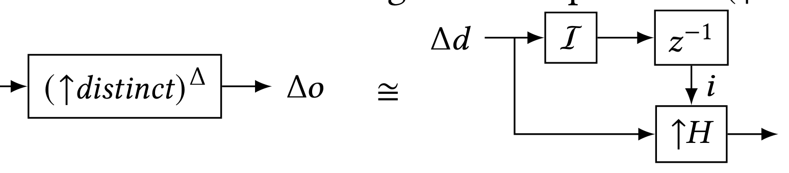
命题 4.7:以下电路实现 $({\uparrow}\mathit{distinct})^\Delta$:
▲ 原文(第 6 页)此处的电路图
其中 $H : \mathbb{Z}[A] \times \mathbb{Z}[A] \to \mathbb{Z}[A]$ 定义为:
$$ H(i, d)[x] \overset{\text{def}}{=} \begin{cases} -1 & \text{若 } i[x] > 0 \text{ 且 } (i + d)[x] \le 0 \\ 1 & \text{若 } i[x] \le 0 \text{ 且 } (i + d)[x] > 0 \\ 0 & \text{否则} \end{cases} $$
FROM ...) I 𝐶𝐼 𝐶𝑂 O 𝐶𝐼 circuit for inner query, 𝐶𝑂 circuit for outer query. Union ( SELECT * FROM I1 )
“$\cong$”右侧的电路把当前的变化 $\Delta d$ 与 $i$(此前所有变化积分后的旧值,经 $z^{-1}$ 延迟一个时间步得到)一起送入提升后的函数 ${\uparrow}H$,由它直接产生输出变化 $\Delta o$。
下面是 $\mathit{distinct}$ 可以被高效增量化的直觉:$({\uparrow}\mathit{distinct})^\Delta$ 的输出中能够出现的元素,必定在输入中已经发生了变化。因此输出变化的大小不会大于输入变化的大小。在上面的电路中,$i$ 是所有变化的积分的前一版本,即正在计算其 $\mathit{distinct}$ 值的那个完整的 $\mathbb{Z}$-集合。函数 $H$ 检测在加上新的增量 $d$ 时,$i$ 中某个元素的权重是否在改变符号(从正变负或反之)。
4.4 增量电路的复杂度4.4 Complexity of incremental circuits
Incremental circuits are efficient. We evaluate the cost of a circuit while processing the 𝑡-th input change. Even if 𝑄 is a pure function, 𝑄Δ is actually a streaming system, with internal state. This state is stored entirely in the delay operators 𝑧−1, some of which appear in I and D operators.
增量电路是高效的。我们在处理第 $t$ 个输入变化时评估一个电路的开销。即使 $Q$ 是纯函数,$Q^\Delta$ 实际上仍是一个带有内部状态的流式系统。这些状态完全存储在延迟算子 $z^{-1}$ 中,其中一部分延迟算子出现在 $\mathcal{I}$ 和 $\mathcal{D}$ 算子内部。$Q^\Delta$ 对第 $t$ 个输入产生的结果,一般不仅取决于新的第 $t$ 个输入,还取决于它此前收到的所有输入。
We argue that each operator in the incremental version of a circuit is efficient in terms of work and space.
我们论证增量版电路中的每个算子在计算量和空间上都是高效的。我们采用标准的 IVM 假设:每个算子的输入变化都很小:
|\Delta DB[t]| \ll |DB[t]| = |(\mathcal{I}(\Delta DB))[t]|
We make the standard IVM assumption that the input changes of each operator are small: |Δ𝐷𝐵 [𝑡]| ≪ |𝐷𝐵 [𝑡]| = |(I (Δ𝐷𝐵)) [𝑡]|. An unoptimized incremental operator 𝑄Δ = D ◦ 𝑄 ◦ I evaluates query 𝑄 on the whole database 𝐷𝐵, the integral of the input stream: 𝐷𝐵 = I (Δ𝐷𝐵); hence its time complexity is the same as that of the non-incremental evaluation of 𝑄. In addition, each of the I and D operators uses 𝑂 (|𝐷𝐵 [𝑡]|) memory.
未经优化的增量算子 $Q^\Delta = \mathcal{D} \circ Q \circ \mathcal{I}$ 在整个数据库 $DB$(输入流的积分)上求值查询 $Q$:$DB = \mathcal{I}(\Delta DB)$;因此它的时间复杂度与非增量地求值 $Q$ 相同。此外,$\mathcal{I}$ 和 $\mathcal{D}$ 算子各自使用 $O(|DB[t]|)$ 的内存。
Step (5) of the incrementalization algorithm applies the optimizations described in §3; these reduce the time complexity of each operator to be a function of 𝑂 (|Δ𝐷𝐵 [𝑡]|). For example, Theorem 3.3, allows evaluating 𝑆Δ, where 𝑆 is a linear operator, in time 𝑂 (|Δ𝐷𝐵 [𝑡]|). The I operator can also be evaluated in 𝑂 (|Δ𝐷𝐵 [𝑡]|) time, because all values that appear in the output of I (Δ𝐷𝐵) [𝑡] must be present in current input change Δ𝐷𝐵 [𝑡]. Similarly, while the distinct operator is not linear, (↑distinct)Δ can also be evaluated in 𝑂 (|Δ𝐷𝐵 [𝑡]|) according to Proposition 4.7.
增量算法中的第 (5) 步应用了 §3 中描述的优化;这些优化把每个算子的时间复杂度降低为 $O(|\Delta DB[t]|)$ 的函数。例如,定理 3.3 允许在时间 $O(|\Delta DB[t]|)$ 内求值 $S^\Delta$,其中 $S$ 是线性算子。$\mathcal{I}$ 算子也可以在 $O(|\Delta DB[t]|)$ 时间内求值,因为 $\mathcal{I}(\Delta DB)[t]$ 输出中出现的所有值必定存在于当前的输入变化 $\Delta DB[t]$ 中。类似地,虽然 $\mathit{distinct}$ 算子不是线性的,但根据命题 4.7,$({\uparrow}\mathit{distinct})^\Delta$ 也可以在 $O(|\Delta DB[t]|)$ 时间内求值。双线性算子(包括连接)可以在时间 $O(|DB[t]| \times |\Delta DB[t]|)$ 内求值,这比完全重新求值要好一个因子 $|DB[t]|/|\Delta DB[t]|$。
Bilinear operators, including join, can be evaluated in time 𝑂 (|𝐷𝐵 [𝑡]| × |Δ𝐷𝐵 [𝑡]|), which is a factor of |𝐷𝐵 [𝑡]/Δ𝐷𝐵 [𝑡]| better than full re-evaluation. The space complexity of linear operators is 0 (zero), since they store no data persistently. The space complexity of operators such as (↑distinct)Δ, (↑ ⊲⊳)Δ, I, and D is 𝑂 (|𝐷𝐵 [𝑡]|). They need to store their input or output relations in full.
线性算子的空间复杂度是 0(零),因为它们不持久存储任何数据。$({\uparrow}\mathit{distinct})^\Delta$、$({\uparrow}\bowtie)^\Delta$、$\mathcal{I}$ 和 $\mathcal{D}$ 这类算子的空间复杂度是 $O(|DB[t]|)$。它们需要完整地存储其输入关系或输出关系。
4.4.1 IVM 查询计划与最优性4.4.1 IVM query plans and optimality. Let us look again at what we
achieved using Algorithm 4.6. A relational algebra query can be implemented by multiple plans, each with a different data-dependent cost4. The input of Algorithm 4.6 is a (relational), non-incremental query plan, produced by a query planner. The algorithm produces an incremental plan that is “similar” to the input plan.
让我们再次审视用算法 4.6 得到了什么。一个关系代数查询可以由多个计划实现,每个计划都有不同的、依赖于数据的代价[^4]。算法 4.6 的输入是一个(关系代数的)非增量查询计划,由查询规划器产生。该算法产生一个与输入计划“相似”的增量计划。
Standard query planners use cost-based heuristics and data statistics to optimize plans. A generic IVM planner does not have this luxury, since the plan must be generated before any data has been fed to the database. Nevertheless, all standard query optimization techniques, perhaps based on historical statistics, can be used to generate the query plan that is supplied to Algorithm 4.6. The question of optimality in the context of IVM plan is a much more difficult topic than optimization of ad-hoc queries, since the chosen IVM plan will execute for all future database updates.
标准的查询规划器使用基于代价的启发式方法和数据统计信息来优化计划。通用的 IVM 规划器没有这种便利,因为计划必须在任何数据被送入数据库之前生成。尽管如此,仍然可以使用所有标准的查询优化技术(也许基于历史统计信息)来生成提供给算法 4.6 的查询计划。在 IVM 计划的语境下,最优性问题比即席查询的优化要困难得多,因为选定的 IVM 计划将在未来的所有数据库更新中执行。
Moreover, since incremental computations maintain internal state, it follows that incremental plans cannot be simply changed in-flight, like we can change ad-hoc queries based on current data statistics: deploying a new plan requires in general constructing its internal state, which is produced by entire history of prior updates. Fortunately, there is a trivial, but somewhat expensive, recipe for installing a new incremental plan: feed the entire current state of the database, as one big change.
此外,由于增量计算维护内部状态,因此增量计划不能像我们可以根据当前数据统计信息更换即席查询那样,在运行途中被简单地更换:部署一个新计划通常需要构造它的内部状态,而该状态是由此前全部更新历史产生的。幸运的是,安装一个新的增量计划有一个简单但多少有些昂贵的办法:把数据库当前的全部状态作为一个大的变化输入进去。
4.5 关系查询示例4.5 Relational Query Example
We apply the IVM algorithm 4.6 to a concrete relational SQL query: CREATE VIEW v AS 4The optimal plan depends not only on the query, but also on the data.
我们把 IVM 算法 4.6 应用到一个具体的关系 SQL 查询上:
CREATE VIEW v AS
SELECT DISTINCT a.x, b.y FROM (
    SELECT t1.x, t1.id FROM t1 WHERE t1.a > 2
) a JOIN (
    SELECT t2.id, t2.y FROM t2 WHERE t2.s > 5
) b ON a.id = b.id
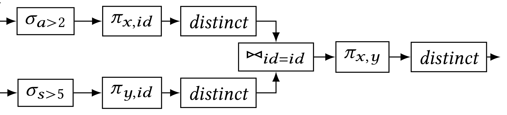
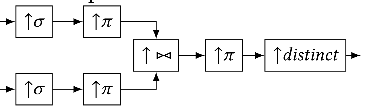
SELECT DISTINCT a . x , b . y FROM ( SELECT t 1 . x , t 1 . i d FROM t 1 WHERE t 1 . a > 2 ) a JOIN ( SELECT t 2 . i d , t 2 . y FROM t 2 WHERE t 2 . s > 5 ) b ON a . i d = b . i d Step 1: Create a DBSP circuit to represent this query using the translation rules from Table 1; notice that this circuit is essentially a dataflow implementation of the query.
第 1 步:使用表 1 中的翻译规则,创建一个 DBSP 电路来表示这个查询;注意,这个电路本质上是该查询的一个数据流实现。(注意该查询要求 SELECT DISTINCT,因此在 $\sigma$ 之后有一个 $\mathit{distinct}$ 算子):
▲ 原文(第 7 页)此处的电路图
第 2 步:应用规则消除 $\mathit{distinct}$ 算子。首先使用命题 4.5:
▲ 原文(第 7 页)此处的电路图
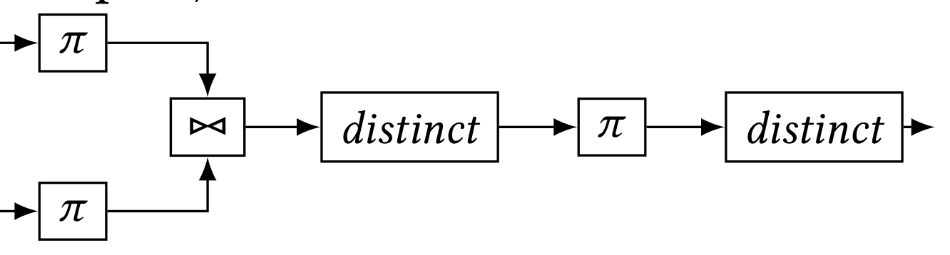
命题 4.4 中的规则给出(从现在起我们省略下标以节省空间):
▲ 原文(第 7 页)此处的电路图
▲ 原文(第 7 页)此处的电路图
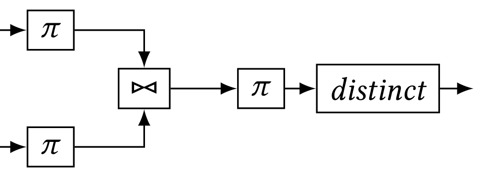
此时已经没有更多的 $\mathit{distinct}$ 消除规则可以应用。
(Notice that the query asks for SELECT DISTINCT, so there is a distinct operator after 𝜎): t1 𝜎𝑎>2 distinct 𝜋𝑥,𝑖𝑑 distinct t2 𝜎𝑠>5 distinct 𝜋𝑦,𝑖𝑑 distinct ⊲⊳𝑖𝑑=𝑖𝑑 𝜋𝑥,𝑦 distinct V Step 2: apply the rules to eliminate distinct operators.
第 3 步:我们利用“复合在提升下满足分配律”(命题 2.4)提升该电路;由此得到一个在流上计算的电路,即:对于每一对新的输入关系 t1 和 t2,它都会产生一个输出视图 V:
▲ 原文(第 7 页)此处的电路图
First from Proposition 4.5: t1 𝜎𝑎>2 𝜋𝑥,𝑖𝑑 distinct t2 𝜎𝑠>5 𝜋𝑦,𝑖𝑑 distinct ⊲⊳𝑖𝑑=𝑖𝑑 𝜋𝑥,𝑦 distinct V The rule from Proposition 4.4 gives (from now on we omit the subscripts to save space): t1 𝜎 𝜋 t2 𝜎 𝜋 ⊲⊳ distinct 𝜋 distinct V And again 4.5: t1 𝜎 𝜋 t2 𝜎 𝜋 ⊲⊳ 𝜋 distinct V At this point no more distinct elimination rules can be applied.
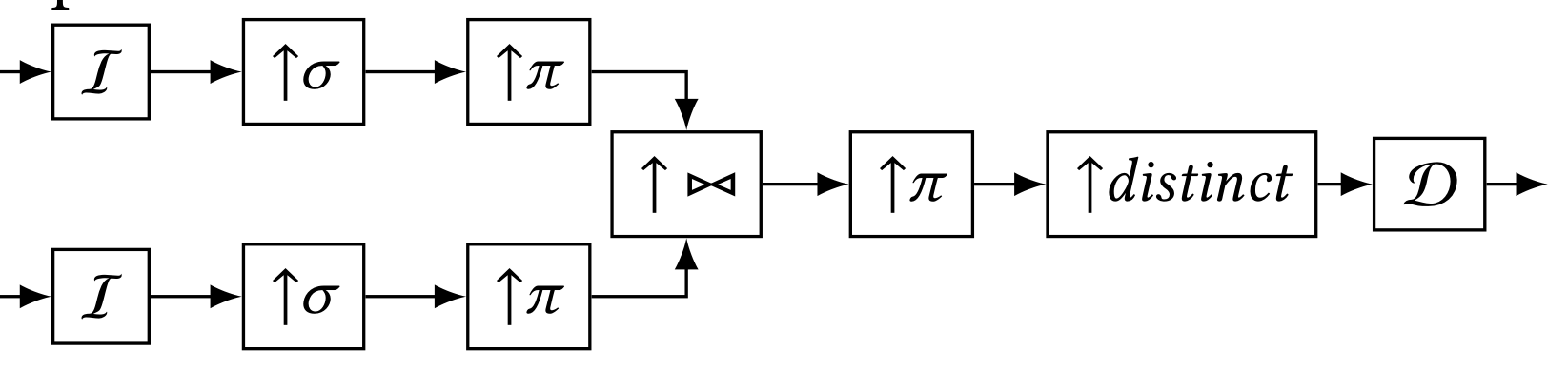
第 4 步:对电路做增量化,得到一个在变化上计算的电路;该电路接收对关系 t1 和 t2 的变化,并对每个这样的变化产生输出视图 V 中相应的变化:
▲ 原文(第 7 页)此处的电路图
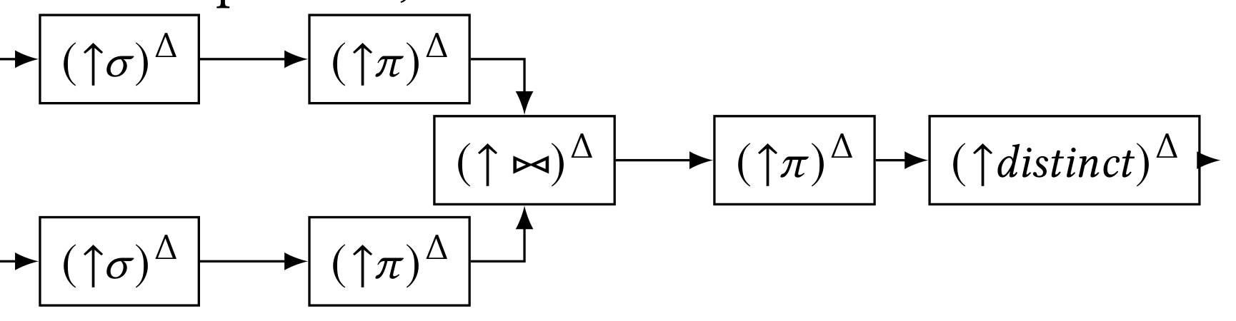
第 5 步:应用链式法则,把电路重写为增量算子的复合:
▲ 原文(第 7 页)此处的电路图
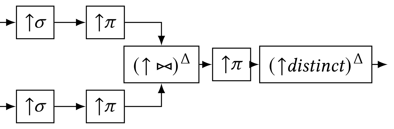
利用 $\sigma$ 和 $\pi$ 的线性来化简该电路(注意所有线性算子不再带有 ${\cdot}^\Delta$):
▲ 原文(第 8 页)此处的电路图
最后,用双线性算子的公式(定理 3.4)替换增量连接,并用命题 4.7 替换增量 $\mathit{distinct}$,得到以下电路。先看各输入分支及其命名的中间值:
Δt1 ──▶ [↑σ] ──▶ [↑π] ──┬──────────────▶ Δa
                        └──▶ [I] ──▶ a

Δt2 ──▶ [↑σ] ──▶ [↑π] ──┬──────────────▶ Δb
                        └──▶ [I] ──▶ [z⁻¹] ──▶ b⁻¹
再由两个连接实例求和得到连接的变化,最后经 $\mathit{distinct}$ 的增量电路产生 $\Delta V$:
▲ 原文(第 8 页)此处的电路图
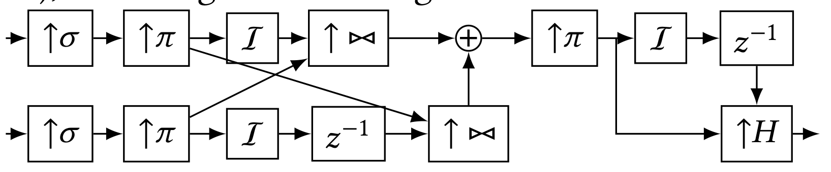
Step 3: we lift the circuit using distributivity of composition over lifting (Proposition 2.4); we obtain a circuit that computes over streams, i.e., for each new input pair of relations t1 and t2 it will produce an output view V: t1 ↑𝜎 ↑𝜋 t2 ↑𝜎 ↑𝜋 ↑ ⊲⊳ ↑𝜋 ↑distinct V Step 4: incrementalize circuit, obtaining a circuit that computes over changes; this circuit receives changes to relations t1 and t2 and for each such change it produces the corresponding change in the output view V: Δt1 I ↑𝜎 ↑𝜋 Δt2 I ↑𝜎 ↑𝜋 ↑ ⊲⊳ ↑𝜋 ↑distinct D ΔV Step 5: apply the chain rule to rewrite the circuit as a composition of incremental operators; Δt1 (↑𝜎)Δ (↑𝜋)Δ Δt2 (↑𝜎)Δ (↑𝜋)Δ (↑ ⊲⊳)Δ (↑𝜋)Δ (↑distinct)Δ ΔV Use the linearity of 𝜎 and 𝜋 to simplify this circuit (notice that all linear operators no longer have a ·Δ): Δt1 ↑𝜎 ↑𝜋 Δt2 ↑𝜎 ↑𝜋 (↑ ⊲⊳)Δ ↑𝜋 (↑distinct)Δ ΔV Finally, replace the incremental join using the formula for bilinear operators (Theorem 3.4), and the incremental distinct (Proposition 4.7), obtaining the following circuit: Δt1 ↑𝜎 ↑𝜋 Δt2 ↑𝜎 ↑𝜋 I I 𝑧−1 ↑ ⊲⊳ ↑ ⊲⊳ + ↑𝜋 I 𝑧−1 ↑𝐻 ΔV Notice that the resulting circuit contains three integration operations: two from the join, and one from the distinct.
其中 $a = \mathcal{I}(\Delta a)$ 与 $b = \mathcal{I}(\Delta b)$ 是两个子查询输出的当前(积分后)值,$b^{-1} = z^{-1}(\mathcal{I}(\Delta b))$ 是 $b$ 延迟一个时间步的旧值,$z^{-1}$ 是延迟算子;两个连接实例之和恰好是定理 3.4 中双线性算子增量公式 $\mathcal{I}(\Delta a) \bowtie \Delta b + \Delta a \bowtie z^{-1}(\mathcal{I}(\Delta b))$ 的两项。$H$ 是命题 4.7 中的符号变化检测函数($i$ 是求和结果经 $\mathcal{I}$、$z^{-1}$ 得到的旧积分值,$d$ 是同一个求和结果本身)。
It also contains two join operators.
注意,所得电路包含三个积分运算:两个来自连接,一个来自 $\mathit{distinct}$。它还包含两个连接算子。然而,每个算子对每个新输入所做的工作量与变化的大小成正比。
However, the work performed by each operator for each new input is proportional to the size of the change.
5 递归查询5 RECURSIVE QUERIES
Recursive queries are very useful in a many applications.
递归查询在许多应用中非常有用。例如,图可达性或传递闭包这类图算法,天然就可以用递归查询来表达。
For example, graph algorithms such as graph reachability or transitive closure are naturally expressed using recursive queries. We introduce two simple DBSP stream operators that are used for expressing recursive query evaluation.
我们引入两个简单的 DBSP 流算子,用于表达递归查询的求值。这些算子使我们能够构造实现循环结构的电路,而循环结构用于反复迭代计算,直到到达一个不动点。
These operators allow us to build circuits implementing looping constructs, which are used to iterate computations until a fixed-point is reached. Definition 5.1: We say that a stream 𝑠 ∈ S𝐴 is zero almosteverywhere if it has a finite number of non-zero values, i.e., there exists a time 𝑡0 ∈ N s.t. ∀𝑡 ≥ 𝑡0.𝑠 [𝑡] = 0. Denote the set of streams that are zero almost everywhere by S𝐴 ⊂ S𝐴. Stream introduction.
定义 5.1(几乎处处为零):称流 $s \in \mathcal{S}_A$ 是几乎处处为零的(zero almost-everywhere),如果它只有有限个非零值,即存在一个时间 $t_0 \in \mathbb{N}$,使得 $\forall t \ge t_0.\ s[t] = 0$。我们把几乎处处为零的流所构成的集合记为 $\overline{\mathcal{S}_A} \subset \mathcal{S}_A$。
The delta function (named from the Dirac delta function) 𝛿0 : 𝐴 → S𝐴 produces a stream from a scalar value: 𝛿0 (𝑣) [𝑡] def ={︃ 𝑣 if 𝑡 = 0 0𝐴 otherwise For example, 𝛿0 (5) is the stream [ 5 0 0 0 0 · · · ].
流引入($\delta_0$):delta 函数(得名于狄拉克 delta 函数)$\delta_0 : A \to \mathcal{S}_A$ 由一个标量值产生一个流:
$$\delta_0(v)[t] \stackrel{\mathrm{def}}{=} \begin{cases} v & \text{若 } t = 0 \\ 0_A & \text{否则} \end{cases}$$
例如,$\delta_0(5)$ 是流 $[\,5\ 0\ 0\ 0\ 0\ \cdots\,]$。
Stream elimination. We define the function ∫ : S𝐴 → 𝐴, over streams that are zero almost everywhere, as ∫ (𝑠) def =∑︁ 𝑡 ≥0 𝑠 [𝑡]. ∫ is closely related to I; if I is the indefinite (discrete) integral, ∫ is the definite (discrete) integral on the interval 0 − ∞. For example,∫ ([ 1 2 3 0 0 · · · ]) = 6.
流消去($\int$):我们在几乎处处为零的流上定义函数 $\int : \mathcal{S}_A \to A$ 为 $\int(s) \stackrel{\mathrm{def}}{=} \sum_{t \ge 0} s[t]$。$\int$ 与 $\mathcal{I}$ 密切相关;如果 $\mathcal{I}$ 是不定(离散)积分,那么 $\int$ 就是区间 $0 - \infty$ 上的定(离散)积分。例如,$\int([\,1\ 2\ 3\ 0\ 0\ \cdots\,]) = 6$。
For many classes of queries (including relational and Datalog queries given below) the ∫ operator can be “approximated” without loss of precision by integrating until the first 0 value encountered.
对于许多类查询(包括下面给出的关系查询与 Datalog 查询),$\int$ 算子都可以“近似”而不损失精度:一直积分到遇到的第一个 0 值为止。
Proposition 5.2: 𝛿0 and ∫ are LTI. Nested time domains.
命题 5.2:$\delta_0$ 与 $\int$ 都是 LTI 的。
So far we have used a tacit assumption that “time” is common for all streams in a program. For example, when we add two streams, we assume that they use the same “clock” for the time dimension. However, the 𝛿0 operator creates a stream with a “new”, independent time dimension.
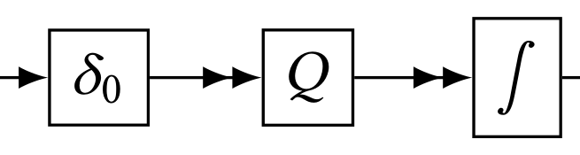
嵌套时间域:到目前为止,我们默认程序中的所有流共享同一个“时间”。例如,当我们把两个流相加时,我们假设它们在时间维上使用同一个“时钟”。然而,$\delta_0$ 算子会创建一个带有“新的”、独立时间维的流。我们要求良构电路(well-formed circuit)把这类嵌套时间域“隔离”开,办法是用 $\delta_0$ 与 $\int$ 算子把它们“括”起来:
▲ 原文(第 8 页)此处的电路图
We require well-formed circuits to “insulate” such nested time domains by “bracketing” them between a 𝛿0 and an ∫ operator: 𝑖 𝛿0 𝑄 ∫ 𝑜 In this circuit the arrows with double heads denote stream values, while the simple arrow denote scalar values5. 𝑄 is a streaming operator, but the entire circuit is a scalar function.
在该电路中,双箭头表示流值,单箭头表示标量值[^5]。$Q$ 是一个流式算子,但整个电路是一个标量函数。
Algorithm 5.3 below, which translates recursive queries to DBSP circuits, always produces well-formed circuits.
下面的算法 5.3 把递归查询翻译为 DBSP 电路,它总是产生良构电路。
5.1 递归查询的实现5.1 Implementing recursive queries
We describe the implementation of recursive queries in DBSP for stratified Datalog. In general, a recursive Datalog program defines a set of mutually recursive relations 𝑂1, .., 𝑂𝑛 as an equation (𝑂1, .., 𝑂𝑛 ) = 𝑅(𝐼1, .., 𝐼𝑚, 𝑂1, .., 𝑂𝑛 ), where 𝐼1, .., 𝐼𝑚 are input relations and 𝑅 is a relational (non-recursive) query.
我们描述 DBSP 中针对分层 Datalog 的递归查询实现。一般而言,一个递归 Datalog 程序把一组相互递归的关系 $O_1,..,O_n$ 定义为一个方程 $(O_1,..,O_n) = R(I_1,..,I_m, O_1,..,O_n)$,其中 $I_1,..,I_m$ 是输入关系,$R$ 是一个关系(非递归)查询。
We describe the algorithm for the simpler case of a single-input, single-output query6. The input of our algorithm is a Datalog query of the form 𝑂 = 𝑅(𝐼, 𝑂), where 𝑅 is a relational, non-recursive query, producing a set as a result, but whose output 𝑂 is also an input. The output of the algorithm is a DBSP circuit which evaluates this recursive query producing output 𝑂 when given the input 𝐼 .
我们针对单输入、单输出查询这个更简单的情形描述该算法[^6]。算法的输入是形如 $O = R(I, O)$ 的 Datalog 查询,其中 $R$ 是一个关系型、非递归的查询,它产生一个集合作为结果,但它的输出 $O$ 同时也是一个输入。算法的输出是一个 DBSP 电路,该电路在给定输入 $I$ 时求值这个递归查询并产生输出 $O$。这里我们构造的是一个非增量电路,它求值该 Datalog 查询;在 §6 中我们将推导该电路的增量版本。
Here we build a non-incremental circuit, which evaluates the Datalog query; in §6 we derive the incremental version of this circuit.
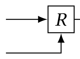
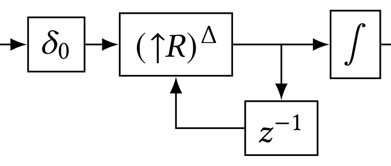
- 按 §4 与表 1 所述,把非递归的关系查询 $R$ 实现出来;这会产生一个无环电路,其输入与输出都是 ℤ-集合:
▲ 原文(第 8 页)此处的电路图
其中 $R$ 的两个输入分别是输入关系 I 与递归关系 O,输出仍是 O。
▲ 原文(第 8 页)此处的电路图
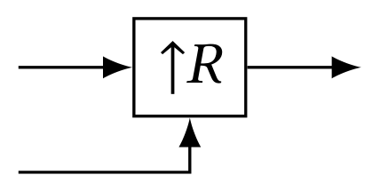
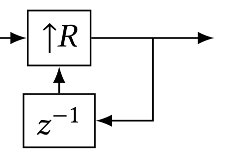
Algorithm 5.3 (recursive queries): (1) Implement the non-recursive relational query 𝑅 as described in §4 and Table 1; this produces an acyclic circuit whose inputs and outputs are a Z-sets: I O 𝑅 O (2) Lift this circuit to operate on streams: I O ↑𝑅 O We construct ↑𝑅 by lifting each operator of the circuit individually according to Proposition 2.4.
我们按照命题 2.4 逐个提升电路中的每个算子来构造 $\uparrow R$。
- 构造一个环,通过一个延迟把输出连接到相应的递归输入:
▲ 原文(第 8 页)此处的电路图
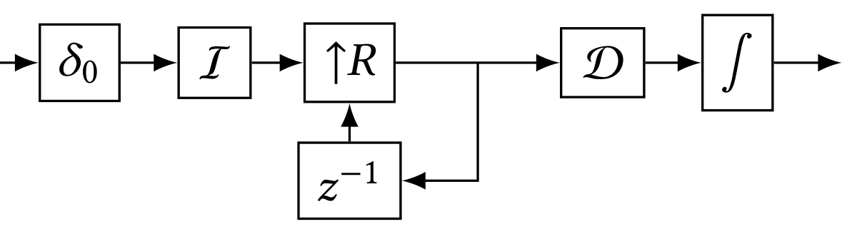
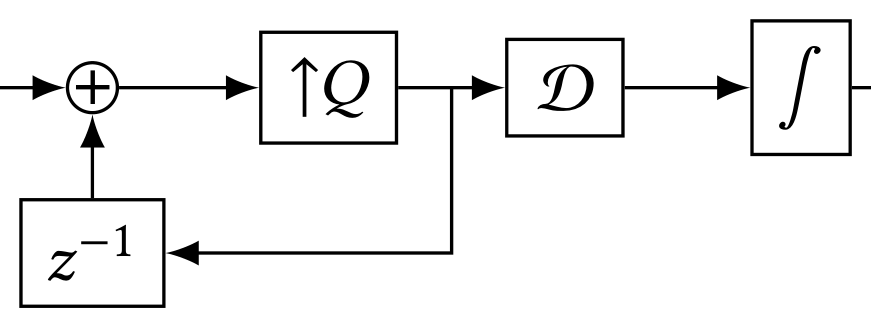
(3) Build a cycle, connecting the output to the corresponding recursive input via a delay: I ↑𝑅 O 𝑧−1 (4) “Bracket” the circuit in I and D nodes, and then in 𝛿0 and ∫ : I 𝛿0 I ↑𝑅 D ∫ O 𝑧−1 We argue that the cycle inside this circuit computes iteratively the fixed point of 𝑅.
- 先用 $\mathcal{I}$ 与 $\mathcal{D}$ 节点、再用 $\delta_0$ 与 $\int$ 把该电路“括”起来:
▲ 原文(第 8 页)此处的电路图
The D operator yields the set of new Datalog facts (changes) computed by each iteration of the loop.
图中 [I] 与 [D] 两个方框分别是积分算子 $\mathcal{I}$ 与微分算子 $\mathcal{D}$,左端不带方框的 I 则是输入关系。
When the set of new facts becomes empty, the fixed point has been reached: Theorem 5.4 (Recursion correctness): If isset(I), the output of the circuit above is the relation O as defined by the Datalog semantics of given program 𝑅 as a function of the input relation I.
我们论证:该电路内部的环迭代地计算 $R$ 的不动点。$\mathcal{D}$ 算子给出循环每一轮迭代所计算出的新 Datalog 事实(即变化)的集合。当新事实的集合变为空时,不动点就已经到达:
Note that if the query 𝑅 computes over unbounded data domains (e.g., using integers with arithmetic), this construction does not guarantee that at runtime a fixed point is reached.
定理 5.4(递归正确性):若 $\mathit{isset}(I)$,则上述电路的输出是关系 O,它由给定程序 $R$ 的 Datalog 语义定义为输入关系 I 的函数。
But if a program 5We only use this convention in this diagram; in general the type of an arrow can be inferred from the type of its source node. 6The general case in the companion technical report [12] is only slightly more involved. does converge, the above construction will find the least fixed point. In fact, this circuit implements the standard naïve evaluation algorithm (e.g., see Algorithm 1 in [21]). Notice that the inner part of the circuit is the incremental form of another circuit, since it is sandwiched between I and D operators.
注意,如果查询 $R$ 在无界数据域上计算(例如使用带算术的整数),则该构造并不保证运行时一定能到达一个不动点。但如果程序确实收敛,上述构造将找到最小不动点。事实上,该电路实现了标准的朴素求值(naïve evaluation)算法(例如见 [21] 中的算法 1)。注意该电路的内层部分是另一个电路的增量形式,因为它被夹在 $\mathcal{I}$ 与 $\mathcal{D}$ 算子之间。利用命题 3.2 的循环规则,我们可以把该电路重写为:
▲ 原文(第 9 页)此处的电路图
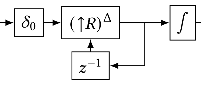
Using the cycle rule of Proposition 3.2 we can rewrite this circuit as: I 𝛿0 (↑𝑅)Δ ∫ O 𝑧−1 (5.1) This circuit implements semi-naïve evaluation (Algorithm 2 from [21]). We have just proven the correctness of semi-naïve evaluation as an immediate consequence of the cycle rule!
该电路实现了半朴素求值(semi-naïve evaluation,[21] 中的算法 2)。我们刚刚证明了半朴素求值的正确性,它正是循环规则的一个直接推论!
6 增量递归程序6 INCREMENTAL RECURSIVE PROGRAMS
In §2–4 we showed how to incrementalize a relational query by compiling it into a circuit, lifting the circuit to compute on streams, and applying the ·Δ operator. In §5 we showed how to compile a recursive query into a circuit that employs incremental computation internally (using semi-naïve evaluation), to compute the fixed point. Here we combine these results to construct a circuit that evaluates a recursive query incrementally. The circuit receives a stream of updates to input relations, and for every update recomputes the fixed point.
在 §2–4 中,我们展示了如何通过把一个关系查询编译成电路、把该电路提升为在流上计算,再施加 $(\cdot)^\Delta$ 算子,来对它做增量化。在 §5 中,我们展示了如何把一个递归查询编译成一个电路,该电路在内部使用增量计算(半朴素求值)来计算不动点。这里我们把这两个结果结合起来,构造一个增量地求值递归查询的电路。该电路接收输入关系上的更新流,并对每一次更新重新计算不动点。为了增量地做到这一点,它保留迭代式不动点计算所产生的、递归关系的变化流,并根据被修改的输入调整这个流。于是,借助嵌套流,输入流的每一个元素都产生一个对不动点计算的调整流。
Thus, every element of the input stream yields a stream of adjustments to the fixed point computation, using nested streams. Nested streams, or streams of streams, SS𝐴 = N → (N → 𝐴), are well defined, since streams form an abelian group. Equivalently, a nested stream is a value in N × N → 𝐴, i.e., a matrix with an infinite number of rows, indexed by two-dimensional time (𝑡0, 𝑡1). where each row is a stream. Please refer to our companion report for example computations on nested streams [12].
嵌套流,即流的流,$\mathcal{S}_{\mathcal{S}_A} = \mathbb{N} \to (\mathbb{N} \to A)$,是良定义的,因为流构成一个阿贝尔群。等价地,嵌套流是 $\mathbb{N} \times \mathbb{N} \to A$ 中的一个值,即一个行数为无限的矩阵,以二维时间 $(t_0,t_1)$ 为索引,其中每一行是一个流。关于嵌套流上的示例计算,请参阅我们的配套报告 [12]。
提升一个流算子 $S : \mathcal{S}_A \to \mathcal{S}_B$ 会得到一个嵌套流上的算子 $\uparrow S : \mathcal{S}_{\mathcal{S}_A} \to \mathcal{S}_{\mathcal{S}_B}$,使得 $(\uparrow S)(s) = S \circ s$;或者按点给出:$(\uparrow S(s))[t_0][t_1] = S(s[t_0])[t_1], \forall t_0,t_1 \in \mathbb{N}$。特别地,一个标量函数 $f : A \to B$ 可以被提升两次,产生一个流之流之间的算子:$\uparrow\uparrow f : \mathcal{S}_{\mathcal{S}_A} \to \mathcal{S}_{\mathcal{S}_B}$。
In particular, a scalar function 𝑓 : 𝐴 → 𝐵 can be lifted twice to produce an operator between streams of streams: ↑↑𝑓 : SS𝐴 → SS𝐵 . To define recursive nested queries, we need a slightly different definition of strictness. If we think of a nested stream 𝐹 : SS𝐴 → SS𝐵 as a function of timestamps (𝑖, 𝑗), then the prior definition of strictness corresponds to strictness in the first dimension 𝑖, which we extend here to allow 𝐹 to be strict in its second dimension 𝑗: for any 𝑠, 𝑠 ′ ∈ SS𝐴 and all times 𝑡 ∈ N, ∀𝑖, 𝑗 < 𝑡 . 𝑠 [𝑖] [ 𝑗] = 𝑠 ′ [𝑖] [ 𝑗] implies 𝐹 (𝑠) [𝑖] [𝑡] = 𝐹 (𝑠 ′) [𝑖] [𝑡]. Proposition 2.9 holds for this extended notion of strictness, i.e., the fixed point operator fix 𝛼 .𝐹 (𝛼) is well defined for a strict operator 𝐹 .
为了定义递归的嵌套查询,我们需要一个略有不同的严格性定义。如果我们把嵌套流 $F : \mathcal{S}_{\mathcal{S}_A} \to \mathcal{S}_{\mathcal{S}_B}$ 看作时间戳 $(i,j)$ 的函数,那么先前的严格性定义对应于在第一个维度 $i$ 上的严格性;我们在此把它扩展为允许 $F$ 在其第二个维度 $j$ 上是严格的:对任意 $s, s' \in \mathcal{S}_{\mathcal{S}_A}$ 和所有时间 $t \in \mathbb{N}$,$\forall i,j < t.\ s[i][j] = s'[i][j]$ 蕴含 $F(s)[i][t] = F(s')[i][t]$。命题 2.9 在这个扩展的严格性概念下成立,即对严格算子 $F$,不动点算子 $\mathrm{fix}\,\alpha.F(\alpha)$ 是良定义的。
命题 6.1:算子 $\uparrow z^{-1} : \mathcal{S}_{\mathcal{S}_A} \to \mathcal{S}_{\mathcal{S}_A}$ 是严格的(在其第二维上)。
Proposition 6.1: The operator ↑𝑧−1 : SS𝐴 → SS𝐴 is strict (in its second dimension). The operator 𝑧−1 on nested streams delays “rows” of the matrix, while ↑𝑧−1 delays “columns”. The I operator on SS𝐴 operates on rows of the matrix, treating each row as a single value. Lifting a stream operator computing on S𝐴, such as I : S𝐴 → S𝐴, also produces an operator on nested streams, but this time computing on the columns of the matrix ↑I : SS𝐴 → SS𝐴 .
嵌套流上的算子 $z^{-1}$ 延迟矩阵的“行”,而 $\uparrow z^{-1}$ 延迟“列”。$\mathcal{S}_{\mathcal{S}_A}$ 上的 $\mathcal{I}$ 算子作用于矩阵的行,把每一行当作一个值。提升一个在 $\mathcal{S}_A$ 上计算的流算子(例如 $\mathcal{I} : \mathcal{S}_A \to \mathcal{S}_A$)也会产生一个嵌套流上的算子,但这次作用于矩阵的列:$\uparrow\mathcal{I} : \mathcal{S}_{\mathcal{S}_A} \to \mathcal{S}_{\mathcal{S}_A}$。
Proposition 6.2 (Lifting cycles): For a binary, causal 𝑇 we have: ↑(𝜆𝑠.fix 𝛼.𝑇 (𝑠, 𝑧−1 (𝛼))) = 𝜆𝑠.fix 𝛼.
命题 6.2(提升环):对二元、因果的 $T$,有:
$$\uparrow(\lambda s.\,\mathrm{fix}\,\alpha.T(s, z^{-1}(\alpha))) = \lambda s.\,\mathrm{fix}\,\alpha.(\uparrow T)(s, (\uparrow z^{-1})(\alpha))$$
(↑𝑇 )(𝑠, (↑𝑧−1)(𝛼)) i.e., lifting a circuit containing a “cycle” can be accomplished by lifting all operators independently, including the 𝑧−1 back-edge.
即:提升一个含有“环”的电路,可以通过独立地提升所有算子(包括 $z^{-1}$ 反馈边)来完成。
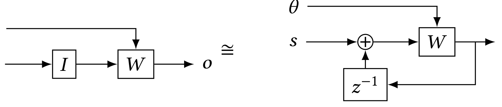
This means that lifting a DBSP stream operator can be expressed within DBSP itself.
这意味着提升一个 DBSP 流算子本身可以在 DBSP 内部表达。例如,我们有:
i ══▶ [ ↑I ] ══▶ o
▲ 原文(第 9 页)此处的电路图
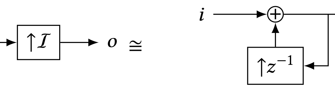
For example, we have: 𝑖 ↑I 𝑜 ≅ 𝑖 + 𝑜 ↑𝑧−1 This proposition gives the ability to lift entire circuits, including circuits computing on streams and having feedback edges, which are well-defined, due to Proposition 6.1.
两者等价($\cong$):右图把 $\uparrow\mathcal{I}$ 表示成一个带反馈的累加器,反馈边上是一个 $\uparrow z^{-1}$ 的延迟。
With this machinery we can now apply Algorithm 4.6 to arbitrary circuits, even circuits built for recursively-defined relations.
该命题使我们能够提升整个电路,包括在流上计算并且带反馈边的电路——由于命题 6.1,这些电路是良定义的。有了这套机制,我们现在可以把算法 4.6 应用于任意电路,甚至是为递归定义的关系而构造的电路。
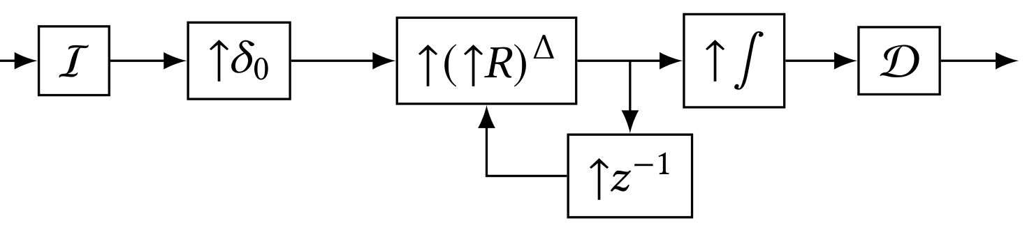
Step 1: Start with the “semi-naive” circuit (5.1): I 𝛿0 (↑𝑅)Δ ∫ O 𝑧−1 Step 2: nothing to do (for distinct).
▲ 原文(第 9 页)此处的电路图
步骤 2:无需做任何事(就 distinct 而言)。
步骤 3 与步骤 4:提升该电路(利用 6.2)并增量化:
▲ 原文(第 9 页)此处的电路图
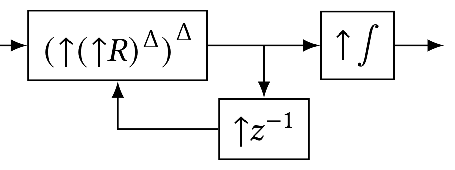
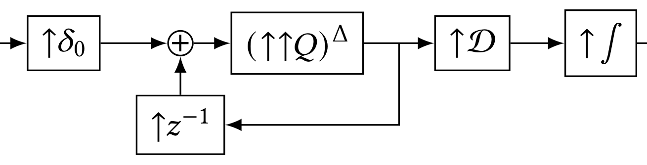
Steps 3 and 4: Lift the circuit (using 6.2) and incrementalize: ΔI I ↑𝛿0 ↑(↑𝑅)Δ ↑ ∫ D ΔO ↑𝑧−1 Step 5: apply the chain rule and linearity of ↑𝛿0 and ↑ ∫ : ΔI ↑𝛿0 (↑(↑𝑅)Δ)Δ ↑ ∫ ΔO ↑𝑧−1 (6.1) This is the incremental version of an arbitrary recursive query.
步骤 5:应用链式法则以及 $\uparrow\delta_0$ 与 $\uparrow\int$ 的线性性:
▲ 原文(第 9 页)此处的电路图
An example for a transitive closure query is in our report [12].
这就是任意递归查询的增量版本。传递闭包查询的一个例子见我们的报告 [12]。
6.1 增量递归查询的代价6.1 Cost of incremental recursive queries
Time complexity. The time complexity of an incremental recursive query can be estimated as a product of the number of fixed point iterations and the complexity of each iteration. The incrementalized circuit (6.1) never performs more iterations than the nonincremental circuit (5.1): once the non-incremental circuit reaches the fixed point, its output is constant, and the derivative of corresponding value in the incrementalized circuit becomes 0. Moreover, the work performed by each operator in the incremental circuit is asymptotically less than the non-incremental one.
时间复杂度。一个增量递归查询的时间复杂度可以估计为不动点迭代次数与每一轮迭代复杂度的乘积。增量化的电路 (6.1) 执行的迭代次数从不多于非增量电路 (5.1):一旦非增量电路到达不动点,它的输出就是常量,而增量化的电路中对应值的导数就变为 0。
A detailed analysis can be found in our companion report [12]. Space complexity.
此外,增量电路中每个算子所做的工作都渐近地少于非增量电路。详细的分析见我们的配套报告 [12]。
Integration (I) and differentiation (D) of a stream Δ𝑠 ∈ SS𝐴 use memory proportional to∑︁ 𝑡2∑︁ 𝑡1 |𝑠 [𝑡1] [𝑡2]|, i.e., the total size of changes aggregated over columns of the matrix. The unoptimized circuit integrates and differentiates respectively inputs and outputs of the recursive program fragment. As we move I and D inside the circuit using the chain rule, we additionally store changes to intermediate streams. Effectively we cache results of fixed point iterations from earlier timestamps to update them efficiently as new input changes arrive.
空间复杂度。对流 $\Delta s \in \mathcal{S}_{\mathcal{S}_A}$ 做积分($\mathcal{I}$)与微分($\mathcal{D}$)所使用的内存正比于 $\sum_{t_2}\sum_{t_1}|s[t_1][t_2]|$,即在矩阵的各列上聚合起来的变化总量。未优化的电路分别对递归程序片段的输入和输出做积分与微分。当我们用链式法则把 $\mathcal{I}$ 与 $\mathcal{D}$ 移到电路内部时,我们还会额外存储对中间流的变化。实际上,我们缓存了较早时间戳上不动点迭代的结果,以便在新的输入变化到来时高效地更新它们。注意,空间占用正比于计算不动点的内层循环的迭代次数。幸运的是,许多递归算法在相当少的步数内就收敛(例如,传递闭包所需的步数是 $\log(\text{图直径})$)。
Notice that space usage is proportional to the number of iterations of the inner loop that computes the fixed-point.
Fortunately, many recursive algorithms converge in a relatively small number of steps (for example, transitive closure requires a number of steps log(graph diameter).
[^6]: 一般情形在我们的配套技术报告 [12] 中,只稍微复杂一些。
7 DBSP 与更丰富的查询语言7 DBSP AND RICHER QUERY LANGUAGES
The DBSP language can express a richer class of streaming computations (both incremental and non-incremental) than those covered so far. In this section we enumerate several important classes of queries that can be implemented in DBSP, and thus can be incrementalized using Algorithm 4.6.
DBSP 语言能够表达比前文所涵盖的更为丰富的一类流计算(既包括增量式的,也包括非增量式的)。本节我们列举若干重要的查询类别,它们都可以在 DBSP 中实现,因而都能用算法 4.6 增量化。
7.1 多重集(bag)7.1 Multisets and bags
In §4 we have shown how to implement the relational algebra on sets. Some SQL queries however produce multisets, e.g., UNION ALL. Since Z-sets generalize multisets and bags, it is trivial to implement query operators on multisets, by just omitting distinct operator invocations. For example, SQL UNION is Z-set addition followed by distinct, whereas UNION ALL is just Z-set addition.
在 §4 中我们展示了如何在集合上实现关系代数。然而有些 SQL 查询产生的是多重集,例如 UNION ALL。由于 ℤ-集合推广了多重集与 bag,在多重集上实现查询算子是很平凡的:只需省略对去重(distinct)算子的调用即可。例如,SQL 的 UNION 是先做 ℤ-集合加法再做去重,而 UNION ALL 只是 ℤ-集合加法。事实上,§8 中提到的 SQL 到 DBSP 编译器处理完整的标准 SQL,包括所有多重集查询。
7.2 聚合7.2 Aggregation
Aggregation in SQL applies a function 𝑎 to a set of values of type 𝐴 producing a “scalar” result with some result type 𝐵: 𝑎 : 2𝐴 → 𝐵. In DBSP an aggregation function has a signature 𝑎 : Z[𝐴] → 𝐵.
SQL 中的聚合把一个函数 $a$ 作用于一个类型为 $A$ 的值集合,产生一个具有某个结果类型 $B$ 的“标量”结果:$a : 2^A \to B$。在 DBSP 中,聚合函数具有签名 $a : \mathbb{Z}[A] \to B$。
The SQL COUNT aggregation function is implemented on Z-sets by 𝑎COUNT : Z[𝐴] → Z, which computes a sum of all the element weights: 𝑎COUNT (𝑠) =∑︁ 𝑥 ∈𝑠 𝑠 [𝑥]. The SQL SUM aggregation function is implemented on Z-sets by 𝑎SUM : Z[R] → R which performs a weighted sum of all (real) values: 𝑎SUM (𝑠) =∑︁ 𝑥 ∈𝑠 𝑥 × 𝑠 [𝑥]. Both these implementations work correctly for sets and multisets. With this definition the aggregation functions 𝑎COUNT and 𝑎SUM are in fact linear transformations between the group Z[𝐴] and the result group (Z, and R respectively).
SQL 的 COUNT 聚合函数在 ℤ-集合上由 $a_{\mathrm{COUNT}} : \mathbb{Z}[A] \to \mathbb{Z}$ 实现,它计算所有元素权重之和:$a_{\mathrm{COUNT}}(s) = \sum_{x \in s} s[x]$。SQL 的 SUM 聚合函数在 ℤ-集合上由 $a_{\mathrm{SUM}} : \mathbb{Z}[\mathbb{R}] \to \mathbb{R}$ 实现,它对所有(实数值)计算加权和:$a_{\mathrm{SUM}}(s) = \sum_{x \in s} x \times s[x]$。这两种实现对于集合与多重集都能正确工作。
If the output of the DBSP circuit is allowed to be such a “scalar” value, then aggregation with a linear function is simply function application, and thus linear.
按照这一定义,聚合函数 $a_{\mathrm{COUNT}}$ 与 $a_{\mathrm{SUM}}$ 实际上是群 $\mathbb{Z}[A]$ 与结果群(分别为 $\mathbb{Z}$ 与 $\mathbb{R}$)之间的线性变换。
However, in general, composing multiple queries requires the result of an aggregation to be a singleton Z-set (containing a single value), and not a scalar value. In this case the aggregation function is implemented in DBSP as the composition of the actual aggregation and the makeset : 𝐴 → Z[𝐴] function, which converts a scalar value of type 𝐴 to a singleton Z-set, defined as follows: makeset(𝑥) def = {𝑥 ↦ → 1}.
如果允许 DBSP 电路的输出就是这样的“标量”值,那么用线性函数做聚合就只是函数应用,因而是线性的。然而一般来说,组合多个查询要求聚合的结果是一个单元素 ℤ-集合(只含一个值),而不是一个标量值。在这种情况下,DBSP 把聚合函数实现为真正的聚合函数与 $\mathrm{makeset} : A \to \mathbb{Z}[A]$ 函数的复合,后者把类型 $A$ 的标量值转换为单元素 ℤ-集合,定义如下:$\mathrm{makeset}(x) \stackrel{\text{def}}{=} \{x \mapsto 1\}$。
In conclusion, the following SQL query: SELECT SUM(c) FROM I is implemented as the following circuit:7 I 𝜋C 𝑎SUM makeset O The lifted incremental version of this circuit is interesting: since 𝜋 and 𝑎SUM are linear, they are equivalent to their own incremental versions.
综上所述,以下 SQL 查询:SELECT SUM(c) FROM I 被实现为如下电路:[^7]
▲ 原文(第 10 页)此处的电路图
Although (↑makeset)Δ = D ◦ ↑makeset ◦ I cannot be simplified, it is nevertheless efficient, doing only O(1) work per invocation, since its input and output are singleton values.
图中 $\pi_{\texttt{C}}$ 是投影算子,$a_{\mathrm{SUM}}$ 是求和聚合函数,$\mathrm{makeset}$ 把标量结果转换为单元素 ℤ-集合。
Finally, some aggregate functions, such as MIN, are not linear: for handling deletions they need to track the full set. One way to implement in DBSP the lifted incremental version of such aggregate 7The actual SQL SUM aggregate is even more complicated, because it needs to skip NULLs, and it returns NULL for an empty input set; this can be implemented in DBSP. functions is by “brute force”, using the formula (↑𝑎MIN)Δ = D ◦ ↑𝑎MIN ◦I.
这个电路的提升增量版本很有意思:由于 $\pi$ 与 $a_{\mathrm{SUM}}$ 都是线性的,它们等价于各自的增量版本。尽管 $({\uparrow}\mathrm{makeset})^{\Delta} = \mathcal{D} \circ {\uparrow}\mathrm{makeset} \circ \mathcal{I}$ 无法化简,但它仍然是高效的:由于它的输入与输出都是单元素值,每次调用只做 $O(1)$ 的工作。
Such an implementations performs work 𝑂 (|𝐷𝐵|) at each invocation. However, schemes such as Reactive Aggregator [47] can be implemented as custom DBSP operators to bring the amortized cost per update to 𝑂 (log |𝐷𝐵|). This approach is similar to the customized implementation of the distinct operator, and it is another facet of the modularity of DBSP, which allows optimized operator implementations to be mixed and matched.
最后,有些聚合函数(例如 MIN)不是线性的:为了处理删除,它们需要跟踪完整的集合。在 DBSP 中实现这类聚合函数的提升增量版本的一种办法是“暴力”地使用公式 $({\uparrow}a_{\mathrm{MIN}})^{\Delta} = \mathcal{D} \circ {\uparrow}a_{\mathrm{MIN}} \circ \mathcal{I}$。这种实现在每次调用时完成 $O(|DB|)$ 的工作。不过,诸如 Reactive Aggregator [47] 这样的方案可以作为自定义 DBSP 算子来实现,从而把每次更新的摊还代价降到 $O(\log |DB|)$。这种做法类似于去重(distinct)算子的定制实现,它也是 DBSP 模块化的又一个侧面:模块化允许把经过优化的算子实现混合搭配使用。
7.3 分组;带索引的关系7.3 Grouping; indexed relations
Let 𝐾 be a set of “key values.” Consider the mathematical structure of finite maps from 𝐾 to Z-sets: 𝐾 → Z[𝐴] = Z[𝐴] [𝐾]. We call values 𝑖 of this structure indexed Z-sets: for each key 𝑘 ∈ 𝐾, 𝑖 [𝑘] is a Z-set. Because the codomain Z[𝐴] is an abelian group, this structure is itself an abelian group. We use this structure to implement the SQL GROUP BY operator in DBSP.
设 $K$ 是一个“键值”的集合。考虑从 $K$ 到 ℤ-集合的有限映射这一数学结构:$K \to \mathbb{Z}[A] = \mathbb{Z}[A][K]$。我们把该结构的取值 $i$ 称为带索引的 ℤ-集合(indexed ℤ-set):对每个键 $k \in K$,$i[k]$ 是一个 ℤ-集合。由于陪域 $\mathbb{Z}[A]$ 是阿贝尔群,这个结构本身也是阿贝尔群。
We define the grouping function 𝐺𝑝 : Z[𝐴] → Z[𝐴] [𝐾] as 𝐺𝑝 (𝑎) [𝑘] def =∑︁ 𝑥 ∈𝑎.𝑝 (𝑥)=𝑘 𝑎[𝑥] · 𝑥 (just map each element of the input 𝑎 to the Z-set grouping corresponding to its key). When applied to a Z-set 𝑎 this function returns a indexed Zset, where each element is a grouping:8 for each key 𝑘 a grouping is a Z-set containing all elements of 𝑎 that map to 𝑘 (as in SQL, groupings are multisets). Consider our example Z-set 𝑅 from §4, and a key function 𝑝 (𝑠) that returns the first letter of the string 𝑠. Then we have that 𝐺𝑝 (𝑅) = {j ↦ → {joe ↦ → 1}, a ↦ → {anne ↦ → −1}}, i.e., grouping with this key function produces an indexed Z-set with two groupings, each of which contains a Z-set with one element.
我们用这个结构在 DBSP 中实现 SQL 的 GROUP BY 算子。考虑一个分区函数(partitioning function)$p : A \to K$,它把 $A$ 中的任意值赋予一个键。我们定义分组函数 $G_p : \mathbb{Z}[A] \to \mathbb{Z}[A][K]$ 为 $G_p(a)[k] \stackrel{\text{def}}{=} \sum_{x \in a.\,p(x)=k} a[x] \cdot x$(即把输入 $a$ 的每个元素映射到其键所对应的 ℤ-集合分组)。当作用于一个 ℤ-集合 $a$ 时,该函数返回一个带索引的 ℤ-集合,其中每个元素是一个分组:[^8] 对每个键 $k$,分组是一个 ℤ-集合,包含 $a$ 中所有映射到 $k$ 的元素(与 SQL 中一样,分组是多重集)。考虑 §4 中我们的示例 ℤ-集合 $R$,以及返回字符串 $s$ 首字母的键函数 $p(s)$。于是有 $G_p(R) = \{\text{j} \mapsto \{\text{joe} \mapsto 1\}, \text{a} \mapsto \{\text{anne} \mapsto -1\}\}$,也就是说,用这个键函数分组产生一个带索引的 ℤ-集合,它有两个分组,其中每个分组都包含一个只有一个元素的 ℤ-集合。
The grouping function 𝐺𝑝 is linear for any key function 𝑝! It follows that the group-by implementation in DBSP is automatically incremental: given some changes to the input relation we can apply the partitioning function to each row changed in the input separately to compute how each grouping changes. Notice that, unlike SQL, DBSP can express naturally computations on indexed Z-sets, they are just an instance of a group structure.
对任意键函数 $p$,分组函数 $G_p$ 都是线性的!由此可知,DBSP 中的 group-by 实现自动就是增量的:给定对输入关系的一些变化,我们可以对输入中发生变化的每一行分别应用分区函数,从而计算出每个分组如何变化。
In DBSP one does not need to follow grouping by aggregation, and DBSP can represent nested groupings of arbitrary depth. Our definition of incremental computation is only concerned with incrementality in the outermost structures. We leave it to future work to explore an appropriate definition of incremental computation on the inner relations.
注意,与 SQL 不同,DBSP 可以自然地表达在带索引的 ℤ-集合上的计算,它们不过是群结构的一个实例。在 DBSP 中不必让分组后面跟着聚合,而且 DBSP 可以表示任意深度的嵌套分组。我们对增量计算的定义只关心最外层结构上的增量性。至于如何在内部关系上定义恰当的增量计算,我们留待未来工作探索。
7.4 GROUP BY-AGGREGATE 与展平映射(flatmap)7.4 GROUP BY-AGGREGATE, flatmap
Grouping in SQL is almost always followed by aggregation. Let us consider an aggregation function 𝑎 : (𝐾 ×Z[𝐴]) → 𝐵 that produces values in some group 𝐵, and an indexed relation of type Z[𝐴] [𝐾], as defined above in §7.3. The nested relation aggregation operator 𝐴𝑔𝑔𝑎 : Z[𝐴] [𝐾] → 𝐵 applies 𝑎 to the contents of each grouping independently and adds the results: 𝐴𝑔𝑔𝑎 (𝑔) def =∑︁ 𝑘 ∈𝐾 𝑎(𝑘, 𝑔[𝑘]).
SQL 中的分组几乎总是后面跟着聚合。考虑一个聚合函数 $a : (K \times \mathbb{Z}[A]) \to B$,它在某个群 $B$ 中产生值;并考虑如上文 §7.3 所定义的类型为 $\mathbb{Z}[A][K]$ 的带索引的关系。嵌套关系聚合算子(nested relation aggregation operator)$Agg_a : \mathbb{Z}[A][K] \to B$ 把 $a$ 独立地作用于每个分组的内容,再把结果相加:$Agg_a(g) \stackrel{\text{def}}{=} \sum_{k \in K} a(k, g[k])$。
To apply this to our example, let us compute the equivalent of GROUP BY-COUNT; we use the following aggregation function 𝑐𝑜𝑢𝑛𝑡 : 𝐾 × Z[𝐴], 𝑐𝑜𝑢𝑛𝑡 (𝑘, 𝑠) = makeset((𝑘, 𝑎COUNT (𝑠))), using the Z-set counting function 𝑎COUNT from §7.2; the notation (𝑎, 𝑏) is a pair of values 𝑎 and 𝑏. Then we have 𝐴𝑔𝑔𝑐𝑜𝑢𝑛𝑡 (𝐺𝑝 (𝑅)) = {(j, 1) ↦ → 8We use “group” for the algebraic structure and “grouping” for the result of GROUP BY. 1, (a, −1) ↦ → 1}.
为了把这个算子应用到我们的示例上,我们来计算 GROUP BY-COUNT 的等价物;我们使用如下聚合函数 $count : K \times \mathbb{Z}[A]$,$count(k, s) = \mathrm{makeset}((k, a_{\mathrm{COUNT}}(s)))$,其中用到 §7.2 的 ℤ-集合计数函数 $a_{\mathrm{COUNT}}$;记号 $(a, b)$ 表示值 $a$ 与 $b$ 构成的二元组。于是有 $Agg_{count}(G_p(R)) = \{(\text{j}, 1) \mapsto 1, (\text{a}, -1) \mapsto 1\}$。
A very useful operation on nested relations is flatmap (or UNNEST in SQL), which is essentially the inverse of grouping, converting an indexed Z-set into a Z-set: flatmap : Z[𝐴] [𝐾] → Z[𝐴 × 𝐾]. flatmap is in fact a particular instance of aggregation, using the aggregation function 𝑎 : 𝐾 × Z[𝐴] → Z[𝐴 × 𝐾] defined by 𝑎(𝑘, 𝑠) =∑︁ 𝑥 ∈𝑠 [𝑘 ] 𝑠 [𝑘] [𝑥] · (𝑘, 𝑥). For our previous example, flatmap(𝐺𝑝 (𝑅)) = {(j, joe) ↦ → 1, (a, anne) ↦ → −1}.
嵌套关系上一个非常有用的操作是展平映射(flatmap),也就是 SQL 中的展开(UNNEST),它本质上是分组的逆操作,把一个带索引的 ℤ-集合转换为一个 ℤ-集合:$\mathrm{flatmap} : \mathbb{Z}[A][K] \to \mathbb{Z}[A \times K]$。flatmap 实际上是聚合的一个特例,它使用的聚合函数 $a : K \times \mathbb{Z}[A] \to \mathbb{Z}[A \times K]$ 定义为 $a(k, s) = \sum_{x \in s[k]} s[k][x] \cdot (k, x)$。对于前面的示例,$\mathrm{flatmap}(G_p(R)) = \{(\text{j}, \text{joe}) \mapsto 1, (\text{a}, \text{anne}) \mapsto -1\}$。
7.5 流连接7.5 Streaming joins
Consider a binary query 𝑇 (𝑠, 𝑡) = I (𝑠) ↑ ⊲⊳ 𝑡. This is the relation-tostream join operator supported by streaming databases like Kafka’s ksqlDB [31]. Stream 𝑠 carries changes to a relation, while 𝑡 carries arbitrary data, e.g., logs or telemetry data points. 𝑇 discards values from 𝑡 after matching them against the accumulated contents of the relation I (𝑠). Streaming Window queries.
考虑一个二元查询 $T(s, t) = \mathcal{I}(s)\;{\uparrow}\!\bowtie\;t$。这是 ksqlDB [31] 这类流式数据库所支持的关系-流连接(relation-to-stream join)算子。流 $s$ 携带对一个关系的变化,而 $t$ 携带任意数据,例如日志或遥测数据点。$T$ 把 $t$ 中的值与关系 $I(s)$ 的累积内容进行匹配,匹配之后就把这些值丢弃。
Streaming databases often organize the contents of streams into windows, which store a subset of data points with a predefined range of timestamps. In practice, windowing is usually based on physical timestamps attached to stream values rather than logical (transaction) time as in the previous circuit. For instance, the CQL [9] query “SELECT * FROM events [RANGE 1 hour]” returns all events received within the last hour.
流式窗口查询(Streaming Window queries)。 流式数据库常常把流的内容组织成窗口,窗口存储具有预定义时间戳范围的一个数据点子集。在实践中,窗口划分通常基于附加在流值上的物理时间戳,而不是像前一个电路那样基于逻辑(事务)时间。例如,CQL [9] 查询 SELECT * FROM events [RANGE 1 hour] 返回过去一小时内收到的所有事件。相应的电路(左图)以流 $s \in \mathcal{S}_{\mathbb{Z}[A]}$ 为输入,并另有一个输入 $\theta \in \mathcal{S}_{\mathbb{R}}$ 携带当前时间的值。
  s ──▶ [ I ] ──▶ [ W ] ──▶ o
                    ▲
  θ ────────────────┘
▲ 原文(第 11 页)此处的电路图
The corresponding circuit (on the left) takes input stream 𝑠 ∈ SZ[𝐴] and an additional input 𝜃 ∈ SR that carries the value of the current time. 𝑠 𝜃 𝐼 𝑊 𝑜 ≅ 𝑠 𝜃 + 𝑊 𝑜 𝑧−1 where the window operator 𝑊 prunes input Z-sets, only keeping values with timestamps less than an hour behind 𝜃 [𝑡].
左图中关系变化流 $s$ 先经积分算子 $\mathcal{I}$ 累积,再经窗口算子 $W$ 修剪;右图把 $W$ 移入积分环路内部:$s$ 与延迟反馈 $z^{-1}$ 相加后进入 $W$,$\theta$ 直接作为 $W$ 的第二个输入,因而只需有界内存。
Assuming 𝑡𝑠 : 𝐴 → R returns the physical timestamp of a value, 𝑊 is defined as 𝑊 (𝑣, 𝜃 ) [𝑡] def = {𝑥 ∈ 𝑣 [𝑡].𝑡𝑠 (𝑥) ≥ 𝜃 [𝑡] − 1ℎ𝑟 }. Assuming 𝜃 increases monotonically, 𝑊 can be moved inside integration, resulting in the circuit on the right, which uses bounded memory to compute a window of an unbounded stream. This circuit is a building block of a large family of window queries, including window joins and window aggregation (e.g., SQL OVER queries).
其中窗口算子 $W$ 修剪输入的 ℤ-集合,只保留时间戳比 $\theta[t]$ 落后不到一小时的取值。假设 $ts : A \to \mathbb{R}$ 返回一个值的物理时间戳,则 $W$ 定义为 $W(v, \theta)[t] \stackrel{\text{def}}{=} \{x \in v[t].\ ts(x) \geq \theta[t] - 1\mathrm{hr}\}$。假设 $\theta$ 单调增长,$W$ 就可以被移到积分内部,从而得到右图电路,它用有界内存计算一个无界流的窗口。这个电路是包括窗口连接与窗口聚合(例如 SQL 的 OVER 查询)在内的一大类窗口查询的构件。
7.6 关系 while 查询7.6 Relational while queries
DBSP can express programs that go beyond Datalog: see the nonmonotonic semantics for Datalog¬ and Datalog¬¬[5].
DBSP 能够表达超出 Datalog 的程序:参见 Datalog$^{\neg}$ 与 Datalog$^{\neg\neg}$ 的非单调语义 [5]。我们实现如下“while”程序,其中 $Q$ 是任意查询:
x := i;
while (x changes)
    x := Q(x);
▲ 原文(第 11 页)此处的电路图
其中 $\delta_0$ 是流引入算子,${\uparrow}Q$ 是提升后的查询 $Q$,$\mathcal{D}$ 与 $\int$ 分别是微分与积分算子,$z^{-1}$ 是延迟算子;反馈边把 ${\uparrow}Q$ 的输出送回加法节点。
We implement the following “while” program, where 𝑄 is an arbitrary query: x := i; while (x changes ) x := Q(x ); The DBSP implementation of this program is: 𝑖 𝛿0 + ↑𝑄 D ∫ 𝑥 𝑧−1 This circuit can be converted to a streaming circuit that computes a stream of values 𝑖 by lifting it; it can be incrementalized using Algorithm 4.6 to compute on changes of 𝑖: Δ𝑖 ↑𝛿0 + (↑↑𝑄)Δ ↑D ↑ ∫ Δ𝑥 ↑𝑧−1 At runtime the execution of this circuit is not guaranteed to terminate; however, if the circuit does terminate, it will produce the correct output, i.e., the least fixpoint of 𝑄 that includes 𝑖.
这个电路可以通过提升转换为计算值 $i$ 的流的流式电路;并且可以用算法 4.6 增量化,以在 $i$ 的变化上进行计算:
▲ 原文(第 11 页)此处的电路图
其中每个算子都是前一个电路中对应算子的(提升后的)增量版本,$(\uparrow\uparrow Q)^{\Delta}$ 是对提升两次的查询再取增量。
在运行时,该电路的执行不保证终止;不过,如果该电路确实终止,它就会产生正确的输出,即 $Q$ 包含 $i$ 的最小不动点。
[^7]: 实际的 SQL SUM 聚合甚至更复杂,因为它需要跳过 NULL,并且对空输入集返回 NULL;这一点可以在 DBSP 中实现。
[^8]: 我们用“群”表示代数结构,用“分组”表示 GROUP BY 的结果。
8 实现8 IMPLEMENTATION
The scope of this paper is the DBSP theory of IVM, so we only briefly touch upon the implementation aspects. We defer a full description and evaluation of the system to a future paper. DBSP Rust library.
本文的范围是 DBSP 的 IVM 理论,因此我们只简要涉及实现方面。我们将系统的完整描述与评估留待后续论文。
The library provides APIs for basic algebraic data types: such as groups, finite maps, Z-set, indexed Z-set. A separate circuit construction API allows users to create DBSP circuits by placing operator nodes (corresponding to boxes in our diagrams) and connecting them with streams, which correspond to the arrows in our diagrams. The library provides prebuilt generic operators for integration, differentiation, delay, nested integration and differentiation, and a rich library of Z-set basic incremental operators: corresponding to plus, negation, grouping, joining, aggregation, distinct, flatmap, window aggregates, etc. For iterative computations the library provides the 𝛿0 operator and an operator that approximates ∫ by terminating iteration of a loop at a user-specified condition (usually the condition is the requirement for a zero to appear in a specified stream). The low level library allows users to construct incremental circuits manually by stitching together incremental versions of primitive operators.
DBSP Rust 库。 我们已作为采用 MIT 许可的开源项目构建了 DBSP 的一个实现:https://github.com/vmware/database-stream-processor。该实现由一个 Rust 库和一个运行时组成。该库为基本代数数据类型提供 API:例如群、有限映射、ℤ-集合(Z-set)、带索引的 ℤ-集合。一个单独的电路构造 API 允许用户通过放置算子节点(对应我们图中的方框)并用流将它们连接起来创建 DBSP 电路,其中流对应我们图中的箭头。该库提供预置的通用算子,用于积分、微分、延迟、嵌套积分与微分,以及一个丰富的 ℤ-集合基本增量算子库:分别对应加、取负、分组、连接、聚合、去重、展平映射(flatmap)、窗口聚合等。对于迭代计算,该库提供 $\delta_0$ 算子,以及一个通过在用户指定条件下终止循环迭代来近似 $\int$ 的算子(通常该条件是要求某个指定流中出现零)。底层库允许用户通过把各基本算子的增量版本拼接起来,手工构造增量电路。该库支持采用一种自然的分片策略对电路进行数据并行的多核求值,并提供多种面向外部数据源(例如 Kafka、CSV 文件等)的适配器。该库还能把算子的内部状态溢写到持久化存储。基准测试结果(非常有前景)可在代码仓库中获得,并将在后续工作中讨论。
We have also built a SQL to DBSP compiler, which translates standard SQL queries into DBSP circuits. The compiler implements Algorithm 4.6, to generate a streaming version of any SQL query. The compiler is open-source https://github.com/vmware/sqlto-dbsp-compiler with an MIT license. The compiler front-end parser and optimizer are based on the Apache Calcite [10] infrastructure.
SQL 编译器。 我们还构建了一个 SQL 到 DBSP 的编译器,它把标准 SQL 查询翻译成 DBSP 电路。该编译器实现了算法 4.6,为任意 SQL 查询生成流式版本。该编译器是开源的,采用 MIT 许可:https://github.com/vmware/sql-to-dbsp-compiler。编译器的前端解析器与优化器基于 Apache Calcite [10] 基础设施。该项目足够成熟,能够通过全部 700 万条 SQL Logic Tests [2]。该编译器处理 SQL 的各个方面,包括 NULL、三值逻辑、分组、聚合、多重集查询等。目前,相关子查询与外连接实质上是使用多个连接转换为等价的关系计划。
Formal verification. We have formalized and verified all the definitions, lemmas, propositions, theorems, and examples in this paper using the Lean theorem prover; we make these proofs available at [14]. The formalization builds on mathlib [37], which provides support for groups and functions with finite support (modeling Zsets). We believe the simplicity of DBSP enabled completing these proofs in relatively few lines of Lean code (5K) and keeping a close correspondence between the paper proofs in [12] and Lean.
形式化验证。 我们使用 Lean 定理证明器对本论文中的所有定义、引理、命题、定理与例子进行了形式化并加以验证;我们把这些证明公开在 [14]。该形式化工作构建在 mathlib [37] 之上,后者提供对群以及具有有限支撑的函数(用于建模 ℤ-集合)的支持。我们相信,正是 DBSP 的简洁性使得这些证明能够以相对较少的 Lean 代码行数(5K)完成,并在 [12] 中的论文证明与 Lean 形式化之间保持密切的对应关系。
9 相关工作9 RELATED WORK
Incremental view maintenance [15, 16, 24–26] is a much studied problem in databases. A survey of results for Datalog queries is present in [40]. The standard approach is as follows: given a query 𝑄, discover a “delta query”, a “differential” version Δ𝑄 that satisfies the equation: 𝑄 (𝑑 +Δ𝑑) = 𝑄 (𝑑) +Δ𝑄 (𝑑, Δ𝑑), and which can be used to compute the change for a new input reusing the previous output. DBToaster introduced recursive recursive IVM [6, 33], where the incrementalization process is repeated for the delta query.
增量视图维护 [15, 16, 24–26] 是数据库领域一个被大量研究的问题。针对 Datalog 查询的结果综述见 [40]。标准方法如下:给定一个查询 $Q$,找出一个“增量查询”(delta query)、即满足方程 $Q(d + \Delta d) = Q(d) + \Delta Q(d, \Delta d)$ 的“微分”版本 $\Delta Q$,它可用于在复用先前输出的同时计算新输入所带来的变化。DBToaster 提出了递归式 IVM(recursive IVM)[6, 33],其中增量化过程会针对增量查询反复执行。
Many custom algorithms were published for various classes of queries: e.g. [34] handles positive nested relational calculus. DYN [28] and IDYN [29, 30] focus on acyclic conjunctive queries. Instead of keeping the output view materialized they build data structures that allow efficiently querying the output views. PAI maps [4] are specially designed for queries with correlated aggregations.
针对各类查询,人们发表了许多定制算法:例如 [34] 处理正嵌套关系演算。DYN [28] 与 IDYN [29, 30] 关注无环合取查询。它们并不把输出视图保持为物化状态,而是构建能够高效查询输出视图的数据结构。PAI maps [4] 专门为带相关聚合的查询设计。AJU [48] 关注外键连接。定制的 DBSP 算子能否达到为窄类查询专门设计的系统的效率,尚待未来工作评估。
AJU [48] focuses on foreign-key joins. It is a matter of future work to evaluate whether custom DBSP operators can match the efficiency of systems specialized for narrow classes of queries. DBSP is a bottom-up system, which always produces eagerly the changes to the output views. Instead of maintaining the output view entirely, DBSP proposes generating deltas as the output of the computation (similar to the kSQL [31] EMIT CHANGES queries).
DBSP 是一个自底向上的系统,它总是急切地(eagerly)产生输出视图的变化。DBSP 不是完整地维护输出视图,而是提出把增量作为计算的输出产生(类似于 kSQL [31] 的 EMIT CHANGES 查询)。IVM 系统的输入与输出都是变化流,这一想法看起来平凡,但它对我们解决方案的对称性至关重要:它既体现在我们对 IVM 的定义(3.1)中,也是链式法则存在的根本原因——正是链式法则使我们的结构归纳 IVM 算法成为可能。
The idea that both inputs and outputs to an IVM system are streams of changes seems trivial, but this is key to the symmetry of our solution: both in our definition of IVM (3.1), and the fundamental reason that the chain rule exists — the chain rule is the one that makes our structural induction IVM algorithm possible. Several IVM algorithms for Datalog-like languages use counting based approaches [19, 41] that maintain the number of derivations of each output fact: DRed [26] and its variants [8, 13, 35, 36, 46, 49], the backward-forward algorithm and variants [27, 40, 41]. DBSP is more general, and our incrementalization algorithm handles arbitrary recursive queries and generates more efficient plans for recursive queries in the presence of arbitrary updates (especially deletions, where competing approaches may over-delete). Interestingly, the Z-sets weights in DBSP are related to the counting-number-ofderivations approaches, but our use of the distinct operator shows that precise counting is not necessary.
若干针对类 Datalog 语言的 IVM 算法采用基于计数的做法 [19, 41],维护每个输出事实的推导(derivation)次数:DRed [26] 及其变体 [8, 13, 35, 36, 46, 49],以及后向-前向算法及其变体 [27, 40, 41]。DBSP 更为一般,我们的增量化算法能处理任意递归查询,并且在存在任意更新(尤其是删除,竞争方法可能会过度删除)的情况下为递归查询生成更高效的执行计划。有趣的是,DBSP 中的 ℤ-集合权重与按推导次数计数的方法相关,但我们使用去重(distinct)算子表明精确计数并非必要。
Picallo et al. [7] provide a general solution to IVM for rich languages. DBSP requires a group structure on the values operated on; this assumption has two major practical benefits: it simplifies the mathematics considerably (e.g., Picallo uses monoid actions to model changes), and it provides a general, simple algorithm (4.6) for incrementalizing arbitrary programs. The downside of DBSP is that one has to find a suitable group structure (e.g., Z-sets for sets) to “embed” the computation.
Picallo 等人 [7] 为富语言中的 IVM 提供了一种通用解决方案。DBSP 要求所操作的值上具有群结构;这一假设有两个主要的实际好处:它极大地简化了数学(例如 Picallo 用幺半群作用(monoid actions)来建模变化),并提供了一个通用而简单的算法(4.6)来增量化任意程序。DBSP 的缺点在于,必须找到一个合适的群结构(例如对集合使用 ℤ-集合)来“嵌入”计算。Picallo 的“导数”(derivative)概念并不唯一:他们需要创造力来选出正确的导数定义,我们需要创造力来找到正确的群结构。
Picallo’s notion of “derivative” is not unique: they need creativity to choose the right derivative definition, we need creativity to find the right group structure. Finding a suitable group structure has proven easy for relations (both [33] and [22] use Z-sets to uniformly model data and insertions/deletions), but it is not obvious how to do it for other data types, such as sorted collections, or tree-shaped collections (e.g., XML or JSON documents) [20]. An intriguing question is “what other interesting group structures could this be applied to besides Z-sets?” Papers such as [43] explore other possibilities, such as matrix algebra, linear ML models, or conjunctive queries.
事实证明,为关系找到合适的群结构很容易([33] 与 [22] 都用 ℤ-集合来统一地建模数据与插入/删除),但对于其他数据类型,例如有序集合或树状集合(如 XML 或 JSON 文档)[20],如何做到这一点并不显然。一个耐人寻味的问题是:“除 ℤ-集合之外,这一方法还能应用到哪些其他有趣的群结构?”诸如 [43] 的论文探索了其他可能性,例如矩阵代数、线性机器学习模型或合取查询。
DBSP does not do anything special for triangle queries [32]. Are there better algorithms for this case?
DBSP 对三角形查询(triangle queries)[32] 没有做任何特殊处理。这一情形是否存在更好的算法?
In §7 we have briefly mentioned that DBSP can easily model window and stream database queries [1, 9]; it is an interesting question whether there are CQL queries that cannot be expressed in DBSP (we conjecture that there aren’t any).
在 §7 中我们简要提到,DBSP 可以很容易地建模窗口与流数据库查询 [1, 9];是否存在无法用 DBSP 表达的 CQL 查询,是一个有趣的问题(我们猜想不存在这类查询)。
Bonifati et al. [11] implemented a verified IVM algorithm for a particular class of graph queries called Regular Datalog, with an implementation machine-checked in the Coq proof assistant. Their focus is on a particular algorithm and the approach does not consider other SQL operators, general recursion, or custom operators (although it is modular in the sense that it works on any query by incrementalizing it recursively). Furthermore, for all queries a deletion in the input change stream requires running the non-incremental query to recover. We formally verify the theorems in our paper, which are much broader in scope, but not our implementations.
Bonifati 等人 [11] 为称为 Regular Datalog 的一类特定图查询实现了一种经过验证的 IVM 算法,其实现用 Coq 证明助手进行了机器检验。他们关注的是某个特定算法,其方法没有考虑其他 SQL 算子、一般递归或定制算子(尽管它是模块化的,即通过对任意查询递归地进行增量化来工作)。此外,对所有查询而言,输入变化流中的一次删除都需要运行非增量查询才能恢复。我们对本文中的定理进行了形式化验证,这些定理的范围要广得多,但我们没有验证自己的实现。
DBSP can express both incremental and non-incremental computations. Most importantly, DBSP comes with Algorithm 4.6, a syntax-directed translation that can convert any expressible query into an incremental version — in DD users have to assemble incremental queries manually using incremental operators. (materialize.com offers a product that automates incrementalization for SQL queries based on DD. Differential Datalog [45] does it for a Datalog dialect.) Unlike DD, DBSP is a modular theory, which easily accommodates the addition of new operators: as long as we can express a new operator as a DBSP circuit, we can (1) define its incremental version, (2) apply the incrementalization algorithm to obtain an efficient incremental implementation, and (3) be confident that it composes with any other operators.
DBSP 也与差分数据流(Differential Dataflow, DD)[39, 42] 及其理论基础 [3](以及近期的 [17, 38])相关。DD 的计算模型比 DBSP 更强大,因为它允许时间值是任意格(lattice)的一部分。事实上,在我们所知的其他框架中,DD 是唯一能像 DBSP 这样高效地增量化递归查询的框架。相比之下,我们的模型要么使用“线性”时间,要么通过模块化提升变换器(${\uparrow}$)使用嵌套时间维度。DBSP 既能表达增量计算,也能表达非增量计算。最重要的是,DBSP 附带算法 4.6——一种语法导向的翻译,能把任何可表达的查询转换为增量版本;而在 DD 中,用户必须使用增量算子手工组装增量查询。(materialize.com 提供了一个基于 DD、为 SQL 查询自动完成增量化的产品。Differential Datalog [45] 则针对一种 Datalog 方言做到这一点。)与 DD 不同,DBSP 是一种模块化的理论,能够轻松容纳新算子的加入:只要能把一个新算子表达为 DBSP 电路,我们就可以 (1) 定义其增量版本,(2) 应用增量化算法得到高效的增量实现,并且 (3) 确信它能与任何其他算子组合。
10 结论10 CONCLUSIONS
We have introduced DBSP, a model of computation based on infinite streams over abelian groups. In this model streams are used for 3 purposes: (1) to model consecutive snapshots of a database, (2) to model consecutive changes (deltas, or transactions) applied to a database and changes of a maintained view, (3) to model consecutive values of loop-carried variables in recursive computations.
我们提出了 DBSP,一种基于阿贝尔群上无限流的计算模型。在该模型中,流用于 3 个目的:(1) 为数据库的连续快照建模;(2) 为施加到数据库上的连续变化(增量或事务)以及被维护视图的变化建模;(3) 为递归计算中循环携带变量的连续取值建模。
We have defined an abstract notion of incremental computation over streams, and defined the incrementalization operator ·Δ, which transforms an arbitrary stream computation 𝑄 into its incremental version 𝑄Δ.
我们定义了流上增量计算的抽象概念,并定义了增量化算子 ${\cdot}^{\Delta}$,它把任意流计算 $Q$ 变换为其增量版本 $Q^{\Delta}$。增量化算子具有一些非常好的代数性质,这些性质为我们提供了一个通用算法,可对许多类复杂查询(包括任意递归查询)进行增量化。
The incrementalization operator has some very nice algebraic properties, which gave us a general algorithm for incrementalizing many classes of complex queries, including arbitrary recursive queries. We believe that DBSP can form a solid foundation for a theory and practice of streaming incremental computation.
我们相信,DBSP 能够为流式增量计算的理论与实践奠定坚实的基础。