高阶语言的变化理论（中英对照）

(front)

面向高阶语言的变化理论——通过静态微分对 λ-演算做增量化（A Theory of Changes for Higher-Order Languages — Incrementalizing λ-Calculi by Static Differentiation）

Yufei Cai、Paolo G. Giarrusso、Tillmann Rendel、Klaus Ostermann

Philipps-Universität Marburg

第 1 页侧栏（ACM 制品徽章）：Consistent* Complete* Well Documented* Easy to Reuse* *Evaluated* PLDI* Artifact* AE

即：该制品在一致性（consistent）、完整性（complete）、文档完善（well documented）、易于复用（easy to reuse）四方面均获认可，并通过了 PLDI 制品评估（Artifact Evaluation, AE）。

摘要

如果一项昂贵计算的结果因输入的微小变化而失效，就应当增量地更新旧结果，而不是重新执行整个计算。我们通过程序的导数来对程序做增量化。导数把程序输入的变化直接映射为程序输出的变化，而无需重新执行原程序。我们给出一项把程序变换为其导数的程序变换，它完全静态、自动，支持一等函数，并且产生的导数可接受标准优化。

我们在一族简单类型 λ-演算上于 Agda 中证明该程序变换是正确的，该族演算以基本类型与原语为参数。一个精确的接口规定了增量化所选原语需要满足什么要求。

我们通过一个案例研究考察性能：我们在 Scala 中实现该程序变换与一个插件，并把一个非平凡程序的性能提升了好几个数量级。

关键词

增量计算、一等函数、性能、Agda、形式化

CCS 分类

Categories and Subject Descriptors：D.1.1 [程序设计技术（Programming Techniques）]：应用式（函数式）编程（Applicative (Functional) Programming）；D.3.3 [程序设计语言（Programming Languages）]：语言构造与特性（Language Constructs and Features）；D.3.4 [程序设计语言（Programming Languages）]：处理器——优化（Processors—Optimization）

ACM 版权行：允许出于个人或课堂使用之目的，对本作品的全部或部分内容制作数字或硬拷贝，无需付费，前提是副本不用于营利或商业优势，且副本须保留本声明与首页的完整引用信息。本作品中由作者之外的他人拥有的组成部分，其版权须予以尊重。允许带出处标注的摘要式使用。以其他方式复制、再出版、在服务器上发布或再分发给邮件列表，均须事先获得专门许可和/或付费。许可申请请联系 permissions@acm.org。

PLDI '14，2014 年 6 月 9–11 日，英国爱丁堡。

版权由作者所有。出版权授予 ACM。

ACM 978-1-4503-2784-8/14/06 ... $15.00

http://dx.doi.org/10.1145/2594291.2594304

1 引言1. Introduction

Incremental computation has a long-standing history in computer science [21]. Often, a program needs to update its output efficiently to reflect input changes [23]. Instead of rerunning such a program from scratch on its updated input, incremental computation research looks for alternatives that are cheaper in a common scenario: namely, when the input change is much smaller than the input itself.

增量计算在计算机科学中有着悠久的历史 [21]。程序常常需要高效地更新其输出，以反映输入的变化 [23]。增量计算研究并不在更新后的输入上从头重跑这样的程序，而是寻找在常见情形下更廉价的替代方案：即输入变化远小于输入本身的情形。

Copyrights for components of this work owned by others than the author(s) must be honored. Abstracting with credit is permitted.

例如，考虑 grand_total 程序，它计算集合（collection）xs、ys 中所有数字之和。

grand_total = λxs. λys. fold (+) 0 (merge xs ys)
output = grand_total {{1, 1}} {{2, 3, 4}} = 11

Now assume that the input xs changes from {{1, 1}} to {{1}}, and ys changes from {{2, 3, 4}} to {{2, 3, 4, 5}}. Instead of recomputing output from scratch, we could also compute it incrementally. If we have a representation for the changes to the inputs (say, dxs = {{remove 1}}, dys = {{add 5}}), we can compute the new result through a function grand _total ′ that takes the old inputs xs = {{1, 1}}, ys = {{2, 3, 4}} and the changes dxs, dys to produce the output change. In this case, it would compute the change grand _total ′ xs dxs ys dys = plus 4, which can then be used to update the original output 11 to yield the updated result 15.

我们用 $\{\!\{\ldots\}\!\}$ 表示多重集（multiset）或 bag，即一种无序集合（类似于集合），其中元素允许出现多次（这一点与集合不同）。现在假设输入 xs 从 $\{\!\{1,1\}\!\}$ 变为 $\{\!\{1\}\!\}$，而 ys 从 $\{\!\{2,3,4\}\!\}$ 变为 $\{\!\{2,3,4,5\}\!\}$。与其从头重新计算 output，我们也可以增量地计算它。如果我们有办法表示输入的变化（例如 dxs = $\{\!\{\mathbf{remove}\ 1\}\!\}$、dys = $\{\!\{\mathbf{add}\ 5\}\!\}$），就可以通过一个函数 grand_total′ 来计算新结果：它接受旧输入 xs = $\{\!\{1,1\}\!\}$、ys = $\{\!\{2,3,4\}\!\}$ 以及变化 dxs、dys，产生输出的变化。在这个例子中，它算出的变化是 grand_total′ xs dxs ys dys = plus 4，这个变化随后可用于把原来的输出 11 更新为更新后的结果 15。我们把 grand_total′ 称为 grand_total 的导数（derivative）。它是与 grand_total 同一门语言中的函数，接受并产生变化，而这些变化是该语言中普通的一等值。若增大原输入 xs、ys 的规模，grand_total xs ys 的时间复杂度线性增长，而 grand_total′ xs dxs ys dys 的时间复杂度只取决于 dxs、dys 的大小；无论在我们的例子中还是在一般情况下，这个大小都更小。

We call grand _total ′ the derivative of grand _total. It is a function in the same language as grand _total, accepting and producing changes, which are simple first-class values of this language.

为了支持自动增量化，本文引入 ILC（incrementalizing λ-calculi）框架。我们定义一个自动的程序变换 $\mathcal{Derive}$，它对程序做微分，即计算程序的导数；$\mathcal{Derive}$ 保证

$$f\,(a \oplus da) \cong (f\,a) \oplus (\mathcal{Derive}(f)\,a\,da). \tag{1}$$

To support automatic incrementalization, in this paper we introduce the ILC (incrementalizing λ-calculi) framework. We define an automatic program transformation Derive that differentiates programs, that is, computes their derivatives; Derive guarantees that f (a ⊕ da) ∼= (f a) ⊕ (Derive(f ) a da) .

其中 $\cong$ 是指称相等（denotational equality），$da$ 是 $a$ 上的一个变化，$a \oplus da$ 表示用变化 $da$ 更新后的 $a$，也就是 $f$ 的更新后的输入。因此，我们可以通过把左边（从头重新计算输出）替换为右边（利用导数增量地计算输出）来优化程序。

(1) where ∼= is denotational equality, da is a change on a and a ⊕ da denotes a updated with change da, that is, the updated input of f . Hence, we can optimize programs by replacing the left-hand side, which recomputes the output from scratch, with the right-hand side, which computes the output incrementally using derivatives.

ILC 基于一个以插件（plugin）为参数的简单类型 λ-演算。一个插件定义 (a) 基本类型与原语操作，以及 (b) 每个基本类型的变化表示，以及每个原语的增量版本。换言之，插件规定了原语及各自的导数，而 ILC 能够把这些简单的导数粘连起来，使得使用这些原语的任意简单类型 λ-演算表达式的导数都可以被计算出来。我们的实现与正确性证明都对插件是参数化的，因此支持（并证明其正确）新的插件很容易。

ILC is based on a simply-typed λ-calculus parameterized by plugins.

本文作出如下贡献：

A plugin defines (a) base types and primitive operations, and (b) a change representation for each base type, and an incremental version for each primitive. In other words, the plugin specifies the primitives and their respective derivatives, and ILC can glue together these simple derivatives in such a way that derivatives for arbitrary simply-typed λ-calculus expressions using these primitives can be computed. Both our implementation and our correctness proof is parametric in the plugins, hence it is easy to support (and prove correct) new plugins. This paper makes the following contributions: • We present a novel mathematical theory of changes and derivatives, which is more general than other work in the field because changes are first-class entities, they are distinct from base values and they are defined also for functions (Sec. 2). • We present the first approach to incremental computation for pure λ-calculi by a source-to-source transformation, Derive, that requires no run-time support.

我们提出一种新的变化与导数的数学理论，它比该领域的其他工作更为一般，因为变化是一等实体，它们与基本值不同，并且也为函数定义了变化（§2）。

The transformation produces an incremental program in the same language; all optimization techniques for the original program are applicable to the incremental program as well. We prove that our incrementalizing145 transformation Derive is correct (Eq. (1)) by a machine-checked formalization in Agda [6]. The proof gives insight into the definition of Derive: we first construct the derivative J − K∆ of the denotational semantics of a simply-typed λ-calculus term, that is, its change semantics. Then, we show that Derive is produced by erasing J − K∆ to a simply-typed program (Sec. 3). • While we focus mainly on the theory of changes and derivatives, we also perform a performance case study.

我们提出第一种针对纯 λ-演算的增量计算方法，它通过源到源变换 $\mathcal{Derive}$ 实现，不需要任何运行时支持。该变换在同一种语言中产生增量程序；原程序的所有优化技术同样适用于增量程序。我们通过在 Agda [6] 中的机器检查形式化，证明我们的增量化变换 $\mathcal{Derive}$ 是正确的（式 (1)）。该证明揭示了 $\mathcal{Derive}$ 的定义思路：我们先构造一个简单类型 λ-演算项的指称语义的导数 $⟦-⟧^{\Delta}$，即其变化语义（change semantics）；然后说明 $\mathcal{Derive}$ 是由 $⟦-⟧^{\Delta}$ 擦除（erasing）为一个简单类型程序而得到的（§3）。

We implement the derivation transformation in Scala, with a plug-in architecture that can be extended with new base types and primitives. We define a plugin with support for different collection types and use the plugin to incrementalize a variant of the MapReduce programming model [16]. Benchmarks show that on this program, incrementalization can reduce asymptotic complexity and can turn O(n) performance into O(1), improving running time by over 4 orders of magnitude on realistic inputs (Sec. 4).

虽然我们主要关注变化与导数的理论，我们也进行了一项性能案例研究。我们在 Scala 中实现了求导变换，其插件式架构可以用新的基本类型与原语来扩展。我们定义了一个支持多种集合类型的插件，并用它来增量化一个 MapReduce 编程模型 [16] 的变体。基准测试表明，在这个程序上，增量化可以降低渐近复杂度，把 $O(n)$ 的性能变为 $O(1)$，在真实输入上把运行时间提高 4 个数量级以上（§4）。

Our Agda formalization, Scala implementation and benchmark results are available at the URL http://inc-lc.github.io/. All lemmas and theorems presented in this paper have been proven in Agda. In the paper, we present an overview of the formalization in more human-readable form, glossing over some technical details.

我们的 Agda 形式化、Scala 实现与基准测试结果可在 http://inc-lc.github.io/ 获取。本文给出的所有引理与定理都已在 Agda 中证明。在本文中，我们以更易读的形式给出形式化的概览，并略过一些技术细节。

2 变化理论2. A theory of changes

This section introduces a formal concept of changes; this concept was already used informally in Eq. (1) and is central to our approach. We first define change structures formally, then construct change structures for functions between change structures, and conclude with a theorem that relates function changes to derivatives.

本节引入变化（change）的形式化概念；这个概念已在式 (1) 中非形式地使用过，并且是我们方法的核心。我们先形式地定义变化结构（change structure），再为变化结构之间的函数构造变化结构，最后以一个把函数变化（function change）与导数联系起来的定理作结。

2.1 变化结构2.1 Change structures

Consider a set of values, for instance the set of natural numbers N. A change dv for v ∈ N should describe the difference between v and another natural vnew ∈ N. We do not define changes directly, but we specify operations which must be defined on them.

考虑一个值的集合，例如自然数集合 $\mathbb{N}$。$v \in \mathbb{N}$ 的一个变化 $dv$ 应当描述 $v$ 与另一个自然数 $v_{new} \in \mathbb{N}$ 之间的差。我们不直接定义变化，而是规定那些必须在变化上定义的运算。它们是：

They are: • We can update a base value v with a change dv to obtain an updated or new value vnew. We write vnew = v ⊕ dv . • We can compute a change between two arbitrary values vold and vnew of the set we are considering. We write dv = vnew vold.

我们可以用一个变化 $dv$ 更新（update）一个基础值 $v$，得到更新后的、或称为新（new）的值 $v_{new}$。我们写作 $v_{new} = v \oplus dv$。

For naturals, it is usual to describe changes using standard subtraction and addition. That is, for naturals we can define v⊕dv = v + dv and vnew vold = vnew − vold.

我们可以计算我们所考虑的集合中任意两个值 $v_{old}$ 与 $v_{new}$ 之间的变化。我们写作 $dv = v_{new} \ominus v_{old}$。

To ensure that ⊕ and are always defined, we need to define the set of changes carefully. N is too small, because subtraction does not always produce a natural; the set of integers Z is instead too big, since adding a natural and an integer does not always produce a natural. In fact, we cannot use the same set of all changes for all naturals. Hence we must adjust the requirements: for each base value v we introduce a set ∆v of changes for v, and require vnew vold to produce values in ∆vold, and v ⊕ dv to be defined for dv in ∆v.

对自然数而言，通常用标准的减法与加法来描述变化。也就是说，对自然数我们可以定义 $v \oplus dv = v + dv$ 以及 $v_{new} \ominus v_{old} = v_{new} - v_{old}$。为了保证 $\oplus$ 与 $\ominus$ 总是有定义，我们需要仔细地定义变化的集合。$\mathbb{N}$ 太小，因为减法并不总产生一个自然数；整数集合 $\mathbb{Z}$ 则太大，因为把一个自然数与一个整数相加并不总产生一个自然数。事实上，我们无法对所有自然数使用同一个包含全部变化的集合。因此我们必须调整要求：对每个基础值 $v$，我们引入 $v$ 的一个变化集合 $\Delta v$，并要求 $v_{new} \ominus v_{old}$ 产生 $\Delta v_{old}$ 中的值，且 $v \oplus dv$ 对 $\Delta v$ 中的 $dv$ 有定义。对自然数 $v$，我们令 $\Delta v = \{\, dv \mid v + dv \ge 0 \,\}$；此时 $\oplus$ 与 $\ominus$ 就总是有定义。

For natural v, we set ∆v = {dv | v + dv ≥ 0}; and ⊕ are then always defined.

下面的定义总结了到此为止的讨论：

The following definition sums up the discussion so far: Definition 2.1 (Change structures). A tuplê V = (V, ∆, ⊕, ) is a change structure (for V ) if: (a) V is a set, called the base set. (b) Given v ∈ V , ∆v is a set, called the change set. (c) Given v ∈ V and dv ∈ ∆v, v ⊕ dv ∈ V .

定义 2.1（变化结构）：一个元组 $\widehat{V} = (V, \Delta, \oplus, \ominus)$ 是（$V$ 上的）一个变化结构，如果：

(a) $V$ 是一个集合，称为基础集合（base set）。 (b) 给定 $v \in V$，$\Delta v$ 是一个集合，称为变化集合（change set）。 (c) 给定 $v \in V$ 与 $dv \in \Delta v$，有 $v \oplus dv \in V$。 (d) 给定 $u, v \in V$，有 $u \ominus v \in \Delta v$。 (e) 给定 $u, v \in V$，$v \oplus (u \ominus v)$ 等于 $u$。

(d) Given u, v ∈ V , u v ∈ ∆v. (e) Given u, v ∈ V , v ⊕ (u v) equals u. One might expect a further assumption that (v ⊕ dv ) v = dv . While it does hold for the change structure of N, it is not needed in general.

人们或许会期望再加一条假设：$(v \oplus dv) \ominus v = dv$。它虽然对 $\mathbb{N}$ 的变化结构成立，但一般并不需要。这意味着多个变化可以表示同一对基础值之间的差。贯穿我们的整个理论，我们只讨论基础值的相等，而不讨论变化的相等。

Notation We overload operators ∆, and ⊕ to refer to the corresponding operations of different change structures; we will subscript these symbols when needed to prevent ambiguity. For anŷ S, we write S for its first component, as above. We make ⊕ left-associative, that is, v ⊕ dv1 ⊕ dv2 means (v ⊕ dv1) ⊕ dv2. We assign precedence to function application over ⊕ and , that is, f a ⊕ g a da means (f a) ⊕ (g a da).

记号我们重载运算符 $\Delta$、$\ominus$ 与 $\oplus$，使它们指代不同变化结构的相应运算；必要时我们会给这些符号加下标以免歧义。对任意 $\widehat{S}$，如上文那样，我们用 $S$ 表示它的第一个分量。我们令 $\oplus$ 左结合，即 $v \oplus dv_1 \oplus dv_2$ 表示 $(v \oplus dv_1) \oplus dv_2$。我们令函数应用的优先级高于 $\oplus$ 与 $\ominus$，即 $f\ a \oplus g\ a\ da$ 表示 $(f\ a) \oplus (g\ a\ da)$。

Examples We demonstrate a change structure on bags with signed multiplicities [15]. These are unordered collections where each element can appear an integer number of times. (a) Let S be any set. The base set V = Bag S is the set of bags of elements of S with signed multiplicities.

例我们展示一个带符号重数的多重集（bag）上的变化结构 [15]。多重集是无序的汇集，其中每个元素可以出现整数次。

The bag {{1, 1, ¯2}} contains two positive occurrences of 1 and a negative occurrence of 2. (b) For each bag v ∈ V , set the change set ∆v = V . Every bag can be a change to any other bag. The bag {{1, 1, ¯5}} represents two insertions of 1 and one deletion of 5.

(a) 令 $S$ 为任意集合。基础集合 $V = \mathrm{Bag}\ S$ 是元素取自 $S$、带符号重数的多重集的集合。多重集 $\{\!\{1, 1, \overline{2}\}\!\}$ 含有两个 $1$ 的正出现与一个 $2$ 的负出现。 (b) 对每个多重集 $v \in V$，令变化集合 $\Delta v = V$。每个多重集都可以是任意其它多重集的变化。多重集 $\{\!\{1, 1, \overline{5}\}\!\}$ 表示两次插入 $1$ 与一次删除 $5$。 (c) 更新运算符是多重集合并：$\oplus = \mathrm{merge}$。两个多重集的合并是重数的逐元素和：

$$\mathrm{merge}\ \{\!\{\overline{1}, 2\}\!\}\ \{\!\{1, 1, \overline{5}\}\!\} = \{\!\{1, 2, \overline{5}\}\!\}.$$

(d) 令 $\mathrm{negate}$ 为对重数取负：

$$\mathrm{negate}\ \{\!\{1, 1, \overline{5}\}\!\} = \{\!\{\overline{1}, \overline{1}, 5\}\!\}.$$

(d) Let negate be the negation of multiplicities: negate {{1, 1, ¯5}} = {{¯1, ¯1, 5}} .

要计算两个多重集的差，就把一个多重集与取负后的多重集合并：

$$u \ominus v = \mathrm{merge}\ u\ (\mathrm{negate}\ v).$$

(e) Given the above definition of ⊕ and , it is not hard to show that v ⊕ (u v) for all bags u, v ∈ V . The change structure we just described is written succinctlŷ Bag S = ( Bag S, (λv. Bag S) , merge, (λx y. merge x (negate y))).

(e) 给定上述 $\oplus$ 与 $\ominus$ 的定义，不难证明对所有多重集 $u, v \in V$ 有 $v \oplus (u \ominus v) = u$。

我们刚才描述的变化结构可以简洁地写作 $\widehat{\mathrm{Bag}}\ S = (\mathrm{Bag}\ S,\ (\lambda v.\ \mathrm{Bag}\ S),\ \mathrm{merge},\ (\lambda x\, y.\ \mathrm{merge}\ x\ (\mathrm{negate}\ y)))$。

This change structure is an instance of a general construction: we can build a change structure from an arbitrary abelian group. An abelian group is a tuple (G, , , e), where is a commutative and associative binary operation, e is its identity element, and produces inverses of elements g of G, such that ( g) g = g ( g) = e. For instance, integers, unlike naturals, form the abelian group (Z, +, −, 0) (where − represents the unary minus). Each abelian group (G, , , e) induces a change structure, namely (G, λg.

这个变化结构是一般构造的一个实例：我们可以从任意的阿贝尔群构造出一个变化结构。阿贝尔群是一个元组 $(G, \boxplus, \boxminus, e)$，其中 $\boxplus$ 是一个可交换且可结合的二元运算，$e$ 是它的单位元，而 $\boxminus$ 产生 $G$ 中元素 $g$ 的逆元，使得 $(\boxminus g) \boxplus g = g \boxplus (\boxminus g) = e$。例如，整数（与自然数不同）构成阿贝尔群 $(\mathbb{Z}, +, -, 0)$（其中 $-$ 表示一元负号）。每个阿贝尔群 $(G, \boxplus, \boxminus, e)$ 都诱导出一个变化结构，即 $(G, \lambda g.\ G, \boxplus, \lambda g\, h.\ g \boxplus (\boxminus h))$，其中任意 $g \in G$ 的变化集合都是整个 $G$。不过，正如自然数的例子所说明的，变化结构更加一般。若 $\varnothing$ 表示空多重集，则 $(\mathrm{Bag}\ S, \mathrm{merge}, \mathrm{negate}, \varnothing)$ 是一个阿贝尔群，它诱导出我们刚才看到的变化结构。

G, , λg h. g ( h)), where the change set for any g ∈ G is the whole G. Change structures are more general, though, as the example with natural numbers illustrates.

整数上的阿贝尔群也在整数上诱导出一个变化结构，即 $\widehat{\mathbb{Z}} = (\mathbb{Z}, (\lambda v.\ \mathbb{Z}), +, -)$。

The abelian group on integers induces also a change structure on integers, namelŷ Z = (Z, (λv.

零变化与导数 一种特别重要的变化是一个值的零变化（nil change）：

Z) , +, −). Nil changes and derivatives A particularly important change is the nil change of a value: Definition 2.2 (Nil change).

定义 2.2（零变化）：给定变化结构 $\widehat{V}$ 与值 $v \in V$，变化 $v \ominus v$ 就是 $v$ 的零变化。

$$\mathbf{0}_v = v \ominus v$$

Given a change structurê V and a value v ∈ V , v ⊕ 0v = v.

值的零变化确实不改变它。

引理 2.3（$\mathbf{0}$ 的行为）：给定变化结构 $\widehat{V}$ 与值 $v \in V$，有 $v \oplus \mathbf{0}_v = v$。

After defining change structures, we can restate the definition of derivatives from Eq. (1).

在定义了变化结构之后，我们可以重新陈述式 (1) 中导数的定义。

Definition 2.4 (Derivatives). Given change structureŝ A and̂ B and a function f ∈ A → B on the change sets of these change structures, we call a binary function f ′ the derivative of f if for all values a ∈ A and corresponding changes da ∈ ∆Aa, f (a ⊕ da) = f a ⊕ f ′ a da.

定义 2.4（导数）：给定变化结构 $\widehat{A}$ 与 $\widehat{B}$，以及这些变化结构的变化集合上的一个函数 $f \in A \to B$，若对所有的值 $a \in A$ 与相应的变化 $da \in \Delta_A a$ 都有

$$f\ (a \oplus da) = f\ a \oplus f'\ a\ da,$$

Applying a derivative to a value and its nil change gives a nil change.

则称二元函数 $f'$ 是 $f$ 的导数（derivative）。

Lemma 2.5 (Behavior of derivatives on 0).

把一个导数作用于一个值及其零变化，得到的是一个零变化。

引理 2.5（导数在 $\mathbf{0}$ 上的行为）：给定变化结构 $\widehat{A}$ 与 $\widehat{B}$、函数 $f \in A \to B$、$A$ 中的元素 $a$，以及 $f$ 的导数 $f'$，我们有 $f'\ a\ \mathbf{0}_a = \mathbf{0}_{(f\ a)}$。

Given change structureŝ A and̂ B, a function f ∈ A → B, an element a of A, and the derivative f ′ of f , we have f ′ a 0a = 0(f a). Examples Let f : Bag S → Bag S be the constant function mapping everything to the empty bag. Its derivative f ′ : Bag S → Bag S → Bag S has to ignore its two arguments and produce the empty bag in all cases.

例令 $f : \mathrm{Bag}\ S \to \mathrm{Bag}\ S$ 为把一切都映射到空多重集的常函数。它的导数 $f' : \mathrm{Bag}\ S \to \mathrm{Bag}\ S \to \mathrm{Bag}\ S$ 必须忽略它的两个参数，并且在所有情形下都产生空多重集。

Let id : Bag S → Bag S be the identity function between bags. Its derivative id ′ is defined by id ′ v dv = dv .

令 $id : \mathrm{Bag}\ S \to \mathrm{Bag}\ S$ 为多重集之间的恒等函数。它的导数 $id'$ 定义为 $id'\ v\ dv = dv$。

2.2 函数变化2.2 Function changes

Allowing values to change is useful, but we need to enable also functions to change. To understand why, think about the curried function grand _total: it takes xs to a function value (closure) knowing the value of xs.

允许值发生变化是有用的，但我们还需要让函数也能发生变化。要理解原因，请考虑柯里化函数 grand_total：它把 xs 映射为一个“知道 xs 的值”的函数值（闭包）。它的导数 grand_total′ 应当满足

$$\texttt{grand\_total}\ (xs \oplus dxs) = \texttt{grand\_total}\ xs \oplus \texttt{grand\_total}'\ xs\ dxs.$$

Similarly, since lambda-calculus functions can also take other functions as arguments, derivatives can take function changes as arguments. In this section, we will demonstrate how we can construct change structures for functions f ∈ A → B, assuming change structures for A and B.

也就是说，grand_total′ 必须把 xs 及其变化映射为一个闭包的变化；用这个变化更新该闭包所得到的结果，必须与 grand_total (xs ⊕ dxs) 相同，也就是一个知道 xs ⊕ dxs 的值的闭包。类似地，既然 λ-演算的函数也可以把其它函数作为参数，导数就可以把函数变化作为参数。

Definitions As seen, the derivative of f computes the change of f a when a becomes a ⊕ da.

本节我们将说明：在假定 $A$ 与 $B$ 的变化结构已给定的前提下，如何为函数 $f \in A \to B$ 构造变化结构。

However, also f can change: As we’ll see in Sec. 3.2, to incrementalize a function application f a we need to compute the difference (f ⊕ df ) (a ⊕ da) f a without rerunning (f ⊕ df ) (a ⊕ da). We compute this difference using function changes, and define change structures on functions precisely to make this possible. A function change df must be a function such that f a ⊕ df a da = (f ⊕ df ) (a ⊕ da) (Theorem 2.9)! Since however f ⊕ df can’t be defined yet, we impose a requirement (Property 2.6b) that we’ll later show equivalent to Theorem 2.9.

定义如前所述，$f$ 的导数计算的是当 $a$ 变为 $a \oplus da$ 时 $f\ a$ 的变化。然而 $f$ 本身也可以变化：正如我们将在 §3.2 看到的，要增量化一次函数应用 $f\ a$，我们需要计算 $(f \oplus df)\ (a \oplus da) \ominus f\ a$ 而不重新运行 $(f \oplus df)\ (a \oplus da)$。我们用函数变化来计算这个差，而之所以精确地在函数上定义变化结构，正是为了使这件事成为可能。函数变化 $df$ 必须是一个满足 $f\ a \oplus df\ a\ da = (f \oplus df)\ (a \oplus da)$ 的函数（定理 2.9）！然而 $f \oplus df$ 目前还无法定义，于是我们施加一项要求（性质 2.6b），稍后我们将说明它与定理 2.9 等价。

Definition 2.6. Given change structureŝ A and̂ B and f ∈ A → B, the set ∆A→B f contains all binary functions df such that (a) df a da ∈ ∆B (f a) and (b) f a ⊕ df a da = f (a ⊕ da) ⊕ df (a ⊕ da) 0(a⊕da) for all values a ∈ A and corresponding changes da ∈ ∆Aa.

定义 2.6：给定变化结构 $\widehat{A}$ 与 $\widehat{B}$ 以及 $f \in A \to B$，集合 $\Delta_{A \to B} f$ 包含所有满足下列条件的二元函数 $df$：

(a) $df\ a\ da \in \Delta_B (f\ a)$，且 (b) $f\ a \oplus df\ a\ da = f\ (a \oplus da) \oplus df\ (a \oplus da)\ \mathbf{0}_{(a \oplus da)}$

Examples Suppose f ∈ Bag S → Bag S and consider a member df of the change set ∆A→B f .

其中 $a \in A$ 取遍所有值，$da \in \Delta_A a$ 取遍相应的变化。

Condition (a) says that df should map a bag and a bag change to another bag change. Condition (b) requires df to mimic the incremental behavior of f . Taken together, they codify what we consider appropriate incremental adjustments to f . In particular, different functions of the same type can have different sets of changes.

例设 $f \in \mathrm{Bag}\ S \to \mathrm{Bag}\ S$，并考虑变化集合 $\Delta_{A \to B} f$ 的一个成员 $df$。条件 (a) 说明 $df$ 应把一个多重集与一个多重集变化映射为另一个多重集变化。条件 (b) 要求 $df$ 模仿 $f$ 的增量式行为。合起来，它们把我们视为对 $f$ 的恰当增量调整编码了下来。

Consider two functions of type Bag S → Bag S. f x = ∅ id x = x The set ∆Bag S→Bag S f contains “changes” to f , namely all binary bag functions df satisfying (b): df a da = df (a ⊕ da) 0(a⊕da) = df (merge a da) ∅.

特别地，同一类型的不同函数可以有不同变化集合。考虑两个类型为 $\mathrm{Bag}\ S \to \mathrm{Bag}\ S$ 的函数。

$$f\ x = \varnothing \qquad\qquad id\ x = x$$

集合 $\Delta_{\mathrm{Bag}\ S \to \mathrm{Bag}\ S} f$ 包含对 $f$ 的“变化”，即所有满足 (b) 的二元多重集函数 $df$：$df\ a\ da = df\ (a \oplus da)\ \mathbf{0}_{(a \oplus da)} = df\ (\mathrm{merge}\ a\ da)\ \varnothing$。这样的二元函数包括 $\mathrm{merge}$ 以及所有常函数。

集合 $\Delta_{\mathrm{Bag}\ S \to \mathrm{Bag}\ S} id$ 包含对 $id$ 的变化，即所有满足 (b) 的二元多重集函数 $did$：$id\ a \oplus did\ a\ da = id\ (a \oplus da) \oplus did\ (a \oplus da)\ \mathbf{0}_{(a \oplus da)}$，它化简为 $\mathrm{merge}\ a\ (did\ a\ da) = \mathrm{merge}\ (\mathrm{merge}\ a\ da)\ (did\ (\mathrm{merge}\ a\ da)\ \varnothing)$。$\mathrm{merge}$ 与任何常函数都不是 $id$ 的变化，但函数 $did\ a\ da = \mathrm{merge}\ da\ \{\!\{1, 2\}\!\}$ 是。

Such binary functions include merge and all constant functions.

函数上的变化结构运算现在可以类似一条分配律来定义。

Neither merge nor any constant function is a change to id, but the function did a da = merge da {{1, 2}} is. The change-structure operations on functions can now be defined similarly to a distributive law. Definition 2.7 (Operations on function changes).

定义 2.7（函数变化上的运算）：给定变化结构 $\widehat{A}$ 与 $\widehat{B}$，运算 $\oplus_{A \to B}$ 与 $\ominus_{A \to B}$ 定义如下。

$$(f \oplus_{A \to B} df)\ v = f\ v \oplus_B df\ v\ \mathbf{0}_v$$

$$(f_2 \ominus_{A \to B} f_1)\ v\ dv = f_2\ (v \oplus_A dv) \ominus_B f_1\ v$$

Given change structureŝ A and̂ B, the operations ⊕A→B and A→B are defined as follows.

所有这些定义都是经过仔细设置的，以确保我们实际上把变化结构提升到了函数空间上。

定理 2.8 给定变化结构 $\widehat{A}$ 与 $\widehat{B}$，元组 $(A \to B, \Delta_{A \to B}, \oplus_{A \to B}, \ominus_{A \to B})$ 是一个变化结构，我们把它记作 $\widehat{A} \to \widehat{B}$。

(f ⊕A→B df ) v = f v ⊕B df v 0v (f2 A→B f1) v dv = f2 (v ⊕A dv ) B f1 v All these definitions have been carefully set up to ensure that we have in fact lifted change structures to function spaces. Theorem 2.8. Given change structureŝ A and̂ B, the tuple (A → B, ∆A→B , ⊕A→B , A→B ) is a change structure, which we denote bŷ A →̂ B.

在定义了这个变化结构之后，我们就可以谈论 $f \oplus df$。于是我们可以重新陈述性质 2.6b，以说明函数变化 $df$ 对输入变化 $da$ 的响应方式与 $f$ 的增量版本相同，也就是说，$df\ a\ da$ 计算的是从 $f\ a$ 到 $(f \oplus df)\ (a \oplus da)$ 的变化：

定理 2.9（增量化）：给定变化结构 $\widehat{A}$ 与 $\widehat{B}$、函数 $f \in A \to B$、值 $a \in A$，以及相应的变化 $df \in \Delta_{A \to B} f$ 与 $da \in \Delta_A a$，我们有

$$(f \oplus df)\ (a \oplus da) = f\ a \oplus df\ a\ da.$$

After defining this change structure, we can talk about f ⊕ df .

例如，把

$$\mathbf{app} = \lambda f.\ \lambda x.\ f\ x$$

So we can restate Property 2.6b to show that a function change df reacts to input changes da like the incremental version of f , that is, df a da computes the change from f a to (f ⊕ df ) (a ⊕ da): Theorem 2.9 (Incrementalization). Given change structureŝ A and̂ B, a function f ∈ A → B and a value a ∈ A with corresponding changes df ∈ ∆A→B f and da ∈ ∆Aa, we have that (f ⊕ df ) (a ⊕ da) = f a ⊕ df a da.

对输入变化 $df$、$dx$ 增量化，就等于在原来的第二个参数 $x_{old}$ 与变化 $dx$ 上调用 $df$。换句话说，把 $\mathbf{app}$ 增量化得到 $\lambda f.\ \lambda df.\ \lambda x.\ \lambda dx.\ df\ x\ dx$。

For instance, incrementalizing app = λf. λx. f x with respect to the input changes df , dx amounts to calling df on the original second argument xold and on the change dx . In other words, incrementalizing app gives λf. λdf . λx. λdx . df x dx . Understanding function changes To understand function changes, we can decompose them into two orthogonal concepts. With a function change df , we can compute at once df aold da, the difference between (f ⊕ df ) (a ⊕ da) and f a, even though both the function and its argument change.

理解函数变化 为了理解函数变化，我们可以把它们分解为两个正交的概念。借助一个函数变化 $df$，我们可以一次计算出 $df\ a_{old}\ da$，即 $(f \oplus df)\ (a \oplus da)$ 与 $f\ a$ 之间的差，即使函数与其参数都在变化。但这两个变化的效果可以分别描述。我们可以用 $f$ 的导数 $f'$ 来刻画 $a$ 的变化：$f\ (a \oplus da) \ominus f\ a = f'\ a\ da$。我们可以用两个函数的逐点差 $\nabla f = \lambda a.\ (f \oplus df)\ a \ominus f\ a$ 来刻画 $f$ 的变化；特别地，$(f \oplus df)\ (a \oplus da) \ominus f\ (a \oplus da) = \nabla f\ (a \oplus da)$。再借助增量化定理，我们就可以说明函数变化不过是一个导数与一个逐点变化的组合：

$$\mathit{fold}\ a_{old} \oplus df\ a_{old}\ da = \mathit{fold}\ a_{old} \oplus f'\ a_{old}\ da \oplus \nabla f\ a_{new}$$

But the effect of those two changes can be described separately.

我们也可以从一个函数变化计算出一个逐点变化：

$$f\ a \oplus df\ a\ \mathbf{0}_a = f\ a \oplus \nabla f\ a$$

We can account for changes to a using f ′, the derivative of f : f (a ⊕ da) f a = f ′ a da.

图 1：我们的基础演算。（原图见 PDF 第 4 页）

We can account for changes to f using the pointwise difference of two functions, ∇f = λa.

（a）语法。 基本类型、类型、类型上下文、常量与项的语法如下。

语法范畴	产生式
基本类型	$\iota ::= \ldots$
类型	$\sigma, \tau ::= \iota \mid \tau \to \tau$
类型上下文	$\Gamma ::= \varepsilon \mid \Gamma, x : \tau$
常量	$c ::= \ldots$
项	$s, t ::= c \mid \lambda x.\ t \mid t\ t \mid x$

(f ⊕ df ) a f a; in particular, (f ⊕ df ) (a ⊕ da) f (a ⊕ da) = ∇f (a ⊕ da).

（b）类型规则。 常量、变量、λ-抽象与应用的类型规则如下。

$$\frac{\ldots}{\vdash c : \tau}\;\mathrm{Const}$$

$$\Gamma_1, x : \tau, \Gamma_2 \vdash x : \tau \qquad \mathrm{Lookup}$$

$$\frac{\Gamma, x : \sigma \vdash t : \tau}{\Gamma \vdash \lambda x.\ t : \sigma \to \tau}\;\mathrm{Lam}$$

$$\frac{\Gamma \vdash s : \sigma \to \tau \qquad \Gamma \vdash t : \sigma}{\Gamma \vdash s\ t : \tau}\;\mathrm{App}$$

(base types) σ, τ ::= ι | τ → τ (types) Γ ::= ε | Γ, x : τ (typing contexts) c ::= . . .

ILC 基于函数变化而不是逐点变化，因为函数变化接收到的信息严格多于逐点变化，因而更易于优化。

2.3 零变化即导数2.3 Nil changes are derivatives

Theorem 2.9 tells us about the form an incremental program may take. If df doesn’t change f at all, that is, if f ⊕ df = f , then Theorem 2.9 becomes f (a ⊕ da) = f a ⊕ df a da.

定理 2.9 告诉我们一个增量程序可以采取的形式。如果 $df$ 根本没有改变 $f$，即如果 $f \oplus df = f$，那么定理 2.9 就变成

$$f\ (a \oplus da) = f\ a \oplus df\ a\ da.$$

It says that df computes the change upon the output of f given a change da upon the input a of f .

它说明：在给定对 $f$ 的输入 $a$ 的一个变化 $da$ 的情况下，$df$ 计算的是 $f$ 的输出上的变化。换句话说，一个函数的零变化正好就是它的导数（见定义 2.4）：

In other words, the nil change to a function is exactly its derivative (see Definition 2.4): Theorem 2.10 (Nil changes are derivatives). Given change structureŝ A and̂ B and a function f ∈ A → B, the change 0f is the derivative f ′ of f .

定理 2.10（零变化即导数）：给定变化结构 $\widehat{A}$ 与 $\widehat{B}$ 以及函数 $f \in A \to B$，变化 $\mathbf{0}_f$ 就是 $f$ 的导数 $f'$。

In this section, we developed the theory of changes to define formally what a derivative is (Definition 2.4) and to recognize that in order to find the derivative of a function, we only have to find its nil change (Theorem 2.10). Next, we want to provide a fully automatic method for finding the nil change of a given function.

本节中，我们发展变化理论，是为了形式地定义什么是导数（定义 2.4），并且认识到：为了求一个函数的导数，我们只需找出它的零变化（定理 2.10）。接下来，我们希望提供一种完全自动的方法，用于找出给定函数的零变化。

3 增量化 λ-演算3. Incrementalizing λ-calculi

In this section, we show how to incrementalize an arbitrary program in simply-typed λ-calculus. To this end, we define the source-tosource transformation Derive. Using the denotational semantics J − K we define later (in Sec. 3.4), we can specify Derive’s intended behavior: to ensure Eq. (1), J Derive(f ) K must be the derivative of J f K for any closed term f : A → B. We will overload the word “derivative” and say simply that Derive(f ) is the derivative of f .

本节我们展示如何增量化简单类型 λ-演算中的任意程序。为此，我们定义源到源的变换 $\mathrm{Derive}$。利用我们稍后（在 §3.4）定义的指称语义 $⟦ - ⟧$，我们可以刻画 $\mathrm{Derive}$ 的预期行为：为保证式 (1) 成立，对任意闭项 $f : A \to B$，$⟦ \mathrm{Derive}(f) ⟧$ 必须是 $⟦ f ⟧$ 的导数。我们将重载“导数”一词，简单地说 $\mathrm{Derive}(f)$ 就是 $f$ 的导数。

It is easy to define derivatives of arbitrary functions as: f ′ x dx = f (x ⊕ dx ) f x.

把任意函数的导数定义为下式是容易的：

$$f'\ x\ dx = f\ (x \oplus dx) \ominus f\ x.$$

We could implement Derive following the same strategy. However, the resulting incremental programs would be no faster than recomputation. We cannot do better for arbitrary mathematical functions, since they are infinite objects which we cannot fully inspect. Therefore, we resort to a source-to-source transformation on simply-typed λ-calculus as defined in Fig. 1.

我们可以按同样的策略实现 $\mathrm{Derive}$。然而，由此得到的增量程序并不会比重新计算更快。对任意数学函数我们无法做得更好，因为它们是我们无法完全检视的无穷对象。因此，我们诉诸于对按图 1 定义的简单类型 λ-演算做源到源变换。本节我们关注所有插件接口实例所共有的那些特性的增量化，即函数类型与相关的语法形式：λ-抽象、应用与变量引用。

Definitions provided by the plugin are replaced, in figures, by ellipses (“. . .”).

基本类型与原始常量的集合，以及原始常量的类型规则，被有意地不加指定，而只由插件定义——它们是扩展点。

Defining different plugins allows to experiment with sets of base types, associated primitives and incrementalization strategies. We summarize requirements on plugins in Sec. 3.7: Satisfying these requirements is sufficient to ensure correct incrementalization. We show an example plugin in our case study (Sec. 4.4). ∆ : ∗ → ∗ the type of changes ⊕ : τ → ∆τ → τ update a value with a change : τ → τ → ∆τ the change between two values

定义不同的插件使我们能够试验不同的基本类型集合、相关原语与增量化策略。我们在 §3.7 中汇总对插件的要求：满足这些要求就足以保证正确的增量化。我们在案例研究（§4.4）中展示一个示例插件。

3.1 变化类型与擦除的变化结构3.1 Change types and erased change structures

We developed the theory of change structures in the previous section to guide our implementation of Derive. By Theorem 2.10, Derive has only to find the nil change to the program itself, because nil changes are derivatives. However, the theory of change structures is not directly applicable to the simply-typed λ-calculus, because a precise implementation of change structures requires dependent types. For instance, we cannot describe the set of changes ∆τ v precisely as a non-dependent type, because it depends on the value we plan to update with these changes.

我们在上一节发展变化结构理论，是为了指导 $\mathrm{Derive}$ 的实现。由定理 2.10，$\mathrm{Derive}$ 只需找出程序自身的零变化，因为零变化就是导数。然而，变化结构理论不能直接应用于简单类型 λ-演算，因为变化结构的精确实现需要依赖类型。例如，我们无法把变化集合 $\Delta\tau\,v$ 精确地描述为一个非依赖类型，因为它依赖于我们计划用这些变化去更新的那个值。

To work around this limitation of our object language, we use a form of erasure of dependent types to simple types. In Fig. 2 and Fig. 4(a), we define change types ∆τ as an approximate description of change sets ∆τ v (Fig. 4(b)). In particular, all changes in ∆τ v correspond to values of terms with type ∆τ , but not necessarily the other way around. For instance, in the change structure for natural numbers described in Sec. 2.1, we would have ∆Nat = Int, even though not every integer is a change for every natural number.

为了绕开我们对象语言的这一局限，我们使用一种把依赖类型擦除为简单类型的形式。在图 2 与图 4(a) 中，我们把变化类型 $\Delta\tau$ 定义为对变化集合 $\Delta\tau\,v$（图 4(b)）的近似描述。特别地，$\Delta\tau\,v$ 中的所有变化都对应类型为 $\Delta\tau$ 的项的值，但反过来不一定成立。例如，在 §2.1 描述的自然数的变化结构中，我们会有 $\Delta\mathbf{Nat} = \mathbf{Int}$，尽管并非每个整数都是每个自然数的变化。对于基本类型 $\iota$，$\Delta\iota$ 及其关联的 $\oplus$ 与 $\ominus$ 算子必须由插件开发者提供。对于函数类型，擦除的变化结构由图 3 给出。把变化结构所有成分中的依赖类型都擦除，我们就得到擦除的变化结构，它把变化结构表示为简单类型 λ-项，其中 $\oplus$ 与 $\ominus$ 是 λ-项的族。

For primitive types ι, ∆ι and its associated ⊕ and operator must be provided by the plugin developer.

图 2：简单类型上的擦除的变化结构。（原图见 PDF 第 4 页）

记号	类型	含义
$\Delta$	$* \to *$	变化的类型
$\oplus$	$\tau \to \Delta\tau \to \tau$	用一个变化更新一个值
$\ominus$	$\tau \to \tau \to \Delta\tau$	两个值之间的变化

For function types, erased change structures are given by Fig. 3.

图 3：函数类型的擦除的变化结构。（原图见 PDF 第 4 页）

$$\Delta(\sigma \to \tau) = \sigma \to \Delta\sigma \to \Delta\tau$$

$$\ominus_{\sigma \to \tau} = \lambda g\, f\, x\, dx.\ (g\,(x \oplus dx)) \ominus (f\, x)$$

$$\oplus_{\sigma \to \tau} = \lambda f\, df\, x.\ (f\, x) \oplus (df\, x\, (x \ominus x))$$

Erasing dependent types in all components of a change structure, we obtain erased change structures, which represent change structures as simply-typed λterms where ⊕ and are families of λ-terms.

图 4：简单类型 λ-演算的标准行为与微分行为。左列把微分定义为源到源的变换；右列定义简单类型 λ-演算的标准语义；中列通过一个微分语义把这两者连接起来，该语义把 λ-项映到其标准语义的导数。（原图见 PDF 第 6 页）

图 4(a) 变化类型：

$$\Delta\iota = \ldots \qquad\qquad \Delta(\sigma \to \tau) = \sigma \to \Delta\sigma \to \Delta\tau$$

图 4(b) 变化值：

$$\Delta\iota\,v = \ldots \subseteq ⟦ \Delta\iota ⟧$$

$$\Delta(\sigma \to \tau)\,f = \{\, df \in (x : ⟦ \sigma ⟧) \to \Delta\sigma\,x \to \Delta\tau\,(f\,x) \mid (f \oplus_{A \to B} df)\,(a \oplus_A da) = f\,a \oplus_B df\,a\,da \,\}$$

图 4(d) 变化上下文：

$$\Delta\varepsilon = \varepsilon \qquad\qquad \Delta(\Gamma, x : \tau) = \Delta\Gamma,\ dx : \Delta\tau$$

Erased change structures are not change structures themselves.

图 4(g) 微分（求导）：

$$\mathrm{Derive}(c) = \ldots$$

$$\mathrm{Derive}(\lambda x.\ t) = \lambda x\, dx.\ \mathrm{Derive}(t)$$

$$\mathrm{Derive}(s\, t) = \mathrm{Derive}(s)\, t\, \mathrm{Derive}(t)$$

$$\mathrm{Derive}(x) = dx$$

However, we will show how change structures and erased changes structures have “almost the same” behavior (Sec. 3.6). We will hence be able to apply our theory of changes.

擦除的变化结构本身并不是变化结构。不过，我们将说明变化结构与擦除的变化结构具有“几乎相同”的行为（§3.6）。因此我们将能够应用我们的变化理论。

3.2 微分3.2 Differentiation

When f is a closed term of function type, Derive(f ) should be its derivative, that is its nil change.

当 $f$ 是函数类型的闭项时，$\mathrm{Derive}(f)$ 应当是其导数，即其零变化。由于 $\mathrm{Derive}$ 在开项上递归，我们需要一个更一般的刻画。我们要求：若 $\Gamma \vdash t : \tau$，则 $\mathrm{Derive}(t)$ 表示 $t$ 的变化（类型为 $\Delta\tau$），且该变化以 $t$ 的自由变量取值的变化为参照。作为一个特例，当 $t$ 是闭项时，没有自由变量可以变化；因此 $t$ 的变化将如所愿地是 $t$ 的零变化。

Since Derive recurses on open terms, we need a more general specification.

下面的类型规则给出 $\mathrm{Derive}$ 的静态语义：

$$\frac{\Gamma \vdash t : \tau}{\Gamma, \Delta\Gamma \vdash \mathrm{Derive}(t) : \Delta\tau}\;\mathrm{Derive}$$

We require that if Γ ` t : τ , then Derive(t) represents the change in t (of type ∆τ ) in terms of changes to the values of its free variables. As a special case, when t is a closed term, there is no free variable to change; hence, the change to t will be, as desired, the nil change of t.148 The following typing rule shows the static semantics of Derive: Γ ` t : τ Γ, ∆Γ ` Derive(t) : ∆τ DERIVE We see that Derive(t) has access both to the free variables in t (from Γ) and to their changes (from ∆Γ, defined in Fig. 4(d)). For example, if a well-typed term t contains x free, then Γ contains an assumption x : τ for some τ and ∆Γ contains the corresponding assumption dx : ∆τ .

我们看到，$\mathrm{Derive}(t)$ 既能访问 $t$ 中的自由变量（来自 $\Gamma$），也能访问它们的变化（来自 $\Delta\Gamma$，定义于图 4(d)）。例如，若良类型的项 $t$ 含有自由变量 $x$，则 $\Gamma$ 含有某个 $\tau$ 的假设 $x : \tau$，而 $\Delta\Gamma$ 含有相应的假设 $dx : \Delta\tau$。因此，$\mathrm{Derive}(t)$ 可以通过使用 $dx$ 访问 $x$ 的变化。为简单起见，我们假设原程序中不含以 $d$ 开头的变量名。$\mathrm{Derive}$ 的定义将保证：若原项是闭的，则 $dx$ 这类变量都被绑定。

Hence, Derive(t) can access the change of x by using dx .

我们来分析 $\mathrm{Derive}(u)$ 的定义（图 4(g)）的各个情形：

For simplicity, we assume that the original program contains no variable names that start with d .

若 $u = x$，则 $\mathrm{Derive}(x)$ 必须是 $x$ 的变化，即 $dx$。

The definition of Derive will ensure that the dx variables are bound if the original term is closed. Let us analyzes each case of the definition of Derive(u) (Fig. 4(g)): • If u = x, Derive(x) must be the change of x, that is dx . • If u = λx. t, Derive(t) is the change of u given the change in its free variables.

若 $u = \lambda x.\ t$，则 $\mathrm{Derive}(t)$ 是在给定其自由变量变化的情形下 $u$ 的变化。$u$ 的变化于是就是 $t$ 作为基础输入 $x$ 及其变化 $dx$ 的函数、相对于其它开变量的变化所发生的变化。因此，我们只需绑定 $dx$，定义 $\mathrm{Derive}(\lambda x.\ t) = \lambda x.\ \lambda dx.\ \mathrm{Derive}(t)$。

The change of u is then the change of t as a function of the base input x and its change dx , with respect to changes in other open variables. Hence, we simply need to bind dx by defining Derive(λx. t) = λx. λdx . Derive(t). • If u = s t, Derive(s) is the change of s as a function of its base input and change.

若 $u = s\, t$，则 $\mathrm{Derive}(s)$ 是 $s$ 作为其基础输入与变化的函数的变化。因此，我们只需把 $\mathrm{Derive}(s)$ 应用于实际的基础输入 $t$ 与变化 $\mathrm{Derive}(t)$，得到 $\mathrm{Derive}(s\, t) = \mathrm{Derive}(s)\, t\, \mathrm{Derive}(t)$。

Hence, we simply apply Derive(s) to the actual base input t and change Derive(t), giving Derive(s t) = Derive(s) t Derive(t). • If t = c: since c is a closed term, its change is a nil change, hence (by Theorem 2.10) c’s derivative. We can obtain a correct derivative for constants by setting: Derive(c) = c c = 0c = c′ This definition is inefficient for functional constants; hence plugins must provide derivatives of the primitives they define. This might seem deceptively simple.

若 $t = c$：由于 $c$ 是闭项，其变化是零变化，从而是（由定理 2.10）$c$ 的导数。我们可以通过令 $\mathrm{Derive}(c) = c \ominus c = \mathbf{0}_c = c'$ 成立来为常量获得正确的导数。该定义对函数型常量效率低下；因此插件必须为其定义的原语提供导数。

But λ-calculus only implements binding of values, leaving “real work” to primitives; likewise, differentiation for λ-calculus only implement binding of changes, leaving “real work” to derivatives of primitives.

这看起来可能简单得具有欺骗性。但 λ-演算只实现值的绑定，把“真正的工作”留给原语；同样，λ-演算的微分只实现变化的绑定，把“真正的工作”留给原语的导数。不过，我们对 λ-演算的支持允许把原语粘在一起。

However, our support for λ-calculus allows to glue the primitives together. Examples Let us apply the transformation on the program grand _total defined in Sec. 1. grand _total = λxs. λys. fold (+) 0 (merge xs ys) Derive(grand _total ) = λxs. λdxs. λys. λdys. fold ′ (+) (+′) 0 0′ (merge xs ys) (merge′ xs dxs ys dys) The names fold ′, merge′, +′, 0′ stand for the derivatives of the corresponding primitives.

例我们把这个变换应用于 §1 中定义的 grand_total 程序。

grand_total = λxs. λys. fold (+) 0 (merge xs ys)

Derive(grand_total) =
  λxs. λdxs. λys. λdys.
    fold′ (+) (+′) 0 0′
      (merge xs ys)
      (merge′ xs dxs ys dys)

The variables dxs and dys are systematically named after xs and ys to stand for their changes. As we shall see in Sec. 3.7, merge′ = λu. λdu. λv. λdv . merge du dv , so the derivative of grand _total is β-equivalent to λxs. λdxs. λys. λdys. fold ′ (+) (+′) 0 0′ (merge xs ys) (merge dxs dys).

名字 fold′、merge′、+′、0′ 分别表示相应原语的导数。变量 dxs 与 dys 依照 xs 与 ys 系统地命名，用来表示它们的变化。正如我们将在 §3.7 看到的，

merge′ = λu. λdu. λv. λdv. merge du dv,

This derivative is inefficient because it needlessly recomputes merge xs ys.

所以 grand_total 的导数 β-等价于

λxs. λdxs. λys. λdys.
  fold′ (+) (+′) 0 0′
    (merge xs ys) (merge dxs dys).

But we still need to inline the derivatives of fold and other primitives to complete derivation. We’ll complete the derivation process and see how to avoid this waste in Sec. 4.3.

这个导数效率低下，因为它不必要地重新计算了 merge xs ys。但我们仍需内联 fold 与其它原语的导数才能完成求导。我们将在 §4.3 完成求导过程，并说明如何避免这种浪费。

We have now informally derived the definition of Derive (Fig. 4(g)) from its specification (Eq. (1)) and its typing. But formally speaking, Derive is instead a definition. So in the rest of this section, we’ll have to prove that Derive satisfies Eq. (1).

我们现在已经从 $\mathrm{Derive}$ 的刻画（式 (1)）与其类型出发，非形式地推导出了 $\mathrm{Derive}$ 的定义（图 4(g)）。但严格说来，$\mathrm{Derive}$ 是一个定义。因此在本节余下部分，我们必须证明 $\mathrm{Derive}$ 满足式 (1)。

3.3 证明的架构3.3 Architecture of the proof

Derive(t) is defined using change types. As discussed in Sec. 3.1, change types impose on their members less restrictions than corresponding change structures – they contain “junk” (such as the change −5 for the natural number 3). We cannot constrain the behavior of Derive(t) on such junk; a direct correctness proof fails. To avoid this problem, our proof defines a version of Derive which uses change structures instead.

$\mathrm{Derive}(t)$ 是借助变化类型定义的。正如 §3.1 所讨论的，变化类型对其成员施加的限制比相应的变化结构更少——它们包含“垃圾”（例如对自然数 3 而言的变化 $-5$）。我们无法约束 $\mathrm{Derive}(t)$ 在这类垃圾上的行为；直接的正确性证明会失败。为避免这个问题，我们的证明定义了一个改用变化结构的 $\mathrm{Derive}$ 版本。

To this end, we first present a standard denotational semantics J − K for simply-typed λ-calculus. Using our theory of changes, we associate change structures to our domains. We define a nonstandard denotational semantics J − K∆, which is analogous to Derive but operates on elements of change structures, so that it needn’t deal with junk.

为此，我们首先给出简单类型 λ-演算的标准指称语义 $⟦ - ⟧$。利用我们的变化理论，我们把变化结构关联到各个论域上。我们定义一个非标准的指称语义 $⟦ - ⟧^{\Delta}$，它类比于 $\mathrm{Derive}$，但在变化结构的元素上运作，从而无需处理垃圾。于是我们可以证明 $⟦ t ⟧^{\Delta}$ 是 $⟦ t ⟧$ 的导数：这是我们的关键结果。

As a consequence, we can prove that J t K∆ is the derivative of J t K: this is our key result. Finally, we define a correspondence between change sets and domains associated with change types, and show that whenever J t K∆ has a certain behavior on an input, J Derive(t) K has the corresponding behavior on the corresponding input. Our correctness property follows as a corollary.

最后，我们定义变化集合与和变化类型相关联的论域之间的对应关系，并说明：每当 $⟦ t ⟧^{\Delta}$ 在某个输入上具有某种行为时，$⟦ \mathrm{Derive}(t) ⟧$ 在对应输入上具有相应的行为。我们的正确性性质作为推论随之成立。

3.4 指称语义3.4 Denotational semantics

In order to prove that incrementalization preserves the meaning of terms, we define a denotational semantics of the object language.

为了证明增量化保持项的含义，我们为对象语言定义一种指称语义。我们首先在插件所提供的基本类型域的基础上，为每个类型关联一个域。由于我们的演算是强规范化的且所有函数都是全函数，我们可以避免用域理论来建模部分性：我们的域就是集合。同样，我们可以用函数作为函数类型的域。

We first associate a domain with every type, given the domains of base types provided by the plugin.

定义 3.1（域）：类型 $\tau$ 的域 $⟦\tau⟧$ 按图 4(c) 定义。

Since our calculus is strongly normalizing and all functions are total, we can avoid using domain theory to model partiality: our domains are simply sets.

有了这种域的构造，我们现在可以为项定义求值函数。常量上的求值函数必须由插件提供。一般地，求值函数 $⟦ t⟧$ 在给定 $t$ 中所有自由变量的值的情况下，计算良类型项 $t$ 的值。自由变量的值由环境提供。

Likewise, we can use functions as the domain of function types.

定义 3.2（环境）：环境 $\rho$ 为自由变量的名字指派值。

$$ \rho ::= \varepsilon \mid \rho, x = v $$

Definition 3.1 (Domains). The domain J τ K of a type τ is defined as in Fig. 4(c).

我们用 $⟦\Gamma⟧$ 表示这样的环境的集合：它们为 $\Gamma$ 中绑定的名字指派值（见图 4(f)）。

Given this domain construction, we can now define an evaluation function for terms. The plugin has to provide the evaluation function for constants.

定义 3.3（求值）：给定 $\Gamma \vdash t : \tau$，$t$ 的含义由图 4(i) 中类型为 $⟦\Gamma⟧ \to ⟦\tau⟧$ 的函数 $⟦ t⟧$ 定义。

In general, the evaluation function J t K computes the value of a well-typed term t given the values of all free variables in t.

这就是简单类型 λ-演算的标准语义。现在我们可以说明，相对这一语义对简单类型 λ-演算做增量化意味着什么。

The values of the free variables are provided in an environment. Definition 3.2 (Environments). An environment ρ assigns values to the names of free variables. ρ ::= ε | ρ, x = v We write J Γ K for the set of environments that assign values to the names bound in Γ (see Fig. 4(f)).

图 4：简单类型 λ-演算的标准行为与微分行为。左栏把微分定义为一个源到源的变换。右栏定义简单类型 λ-演算的标准语义。中栏通过一个微分语义把这两者连接起来，该语义把 λ-项映射到其标准语义的导数。（原图为 3 栏 × 3 行的网格，子图编号为 (a)–(i)；下文按左、中、右三栏依次列出。原图见 PDF 第 6 页）

Definition 3.3 (Evaluation).

左栏：微分（源到源的变换）

(a) 变化类型

$$ \begin{aligned} \Delta\iota &= \ldots\\ \Delta(\sigma \to \tau) &= \sigma \to \Delta\sigma \to \Delta\tau \end{aligned} $$

(d) 变化上下文

$$ \begin{aligned} \Delta\varepsilon &= \varepsilon\\ \Delta(\Gamma, x{:}\tau) &= \Delta\Gamma, dx : \Delta\tau \end{aligned} $$

(g) 微分

$$ \begin{aligned} \mathcal{Derive}(c) &= \ldots\\ \mathcal{Derive}(\lambda x.\, t) &= \lambda x\, dx.\ \mathcal{Derive}(t)\\ \mathcal{Derive}(s\ t) &= \big(\mathcal{Derive}(s)\ t\big)\ \mathcal{Derive}(t)\\ \mathcal{Derive}(x) &= dx \end{aligned} $$

中栏：变化值、变化环境与微分求值（变化语义）

(b) 变化值，其中 $dv, df \in \Delta\tau\, v$

$$ \begin{aligned} \Delta\iota\, v &= \ldots \subseteq ⟦ \Delta\iota ⟧\\ \Delta(\sigma \to \tau)\, f &= \Big\{\, df \in (x : ⟦\sigma⟧) \to \Delta\sigma\, x \to \Delta\tau\, (f\, x) \;\Big|\; \\ &\qquad (f \oplus_{A \to B} df)\ (a \oplus_A da) = (f\, a) \oplus_B (df\, a\ da) \,\Big\} \end{aligned} $$

(e) 变化环境，其中 $d\rho \in \Delta\Gamma\, \rho$；$\rho \in ⟦\Gamma⟧$

$$ \begin{aligned} \Delta\varepsilon\, \emptyset &= \{\emptyset\}\\ \Delta(\Gamma, x{:}\tau)\, (\rho, x{=}v) &= \big\{\, (d\rho, dx{=}dv) \mid d\rho \in \Delta\Gamma\, \rho \;\wedge\; dv \in \Delta\tau\, v \,\big\} \end{aligned} $$

(h) 微分求值，其中 $⟦ t⟧^{\Delta} \rho\, d\rho$

$$ \begin{aligned} ⟦ c ⟧^{\Delta} \rho\, d\rho &= \ldots\\ ⟦ \lambda x.\, t ⟧^{\Delta} \rho\, d\rho &= \lambda v\, dv.\ ⟦ t ⟧^{\Delta}\, (\rho, x{=}v)\ (d\rho, dx{=}dv)\\ ⟦ s\ t ⟧^{\Delta} \rho\, d\rho &= \Big(\big(⟦ s ⟧^{\Delta} \rho\, d\rho\big)\ \big(⟦ t ⟧ \rho\big)\Big)\ \big(⟦ t ⟧^{\Delta} \rho\, d\rho\big)\\ ⟦ x ⟧^{\Delta} \rho\, d\rho &= \mathit{lookup}\ dx\ \text{in}\ d\rho \end{aligned} $$

右栏：标准值、标准环境与标准求值

Given Γ ` t : τ , the meaning of t is defined by the function J t K of type J Γ K → J τ K in Fig. 4(i).

$$ \begin{aligned} ⟦\iota⟧ &= \ldots\\ ⟦\sigma \to \tau⟧ &= ⟦\sigma⟧ \to ⟦\tau⟧ \end{aligned} $$

This is the standard semantics of the simply-typed λ-calculus.

(f) 标准环境，其中 $\rho \in ⟦\Gamma⟧$

$$ \begin{aligned} ⟦\varepsilon⟧ &= \{\emptyset\}\\ ⟦\Gamma, x{:}\tau⟧ &= \big\{\, (\rho, x{=}v) \mid \rho \in ⟦\Gamma⟧ \;\wedge\; v \in ⟦\tau⟧ \,\big\} \end{aligned} $$

We can now specify what it means to incrementalize the simplytyped λ calculus with respect to this semantics.

(i) 标准求值，其中 $⟦ t⟧\, \rho$

$$ \begin{aligned} ⟦ c ⟧ \rho &= \ldots\\ ⟦ \lambda x.\, t ⟧ \rho &= \lambda v.\ ⟦ t ⟧\, (\rho, x{=}v)\\ ⟦ s\ t ⟧ \rho &= \big(⟦ s ⟧ \rho\big)\ \big(⟦ t ⟧ \rho\big)\\ ⟦ x ⟧ \rho &= \mathit{lookup}\ x\ \text{in}\ \rho \end{aligned} $$

3.5 变化语义3.5 Change semantics

The informal specification of differentiation is to map changes in a program’s input to changes in the program’s output. In order to formalize this specification in terms of change structures and the denotational semantics of the object language, we now define a non-standard denotational semantics of the object language that computes changes. The evaluation function J t K∆ computes how the value of a well-typed term t changes given both the values and149 ∆τ dv , df ∈ ∆τ v v, f ∈ J τ K ∆ι = . . . ∆ (σ → τ ) = σ → ∆σ → ∆τ ∆ιv = . . . ⊆ J ∆ι K ∆(σ→τ )f = {df ∈ (x : J σ K) → ∆σ x → ∆τ (f x) | (f ⊕A→B df ) (a ⊕A da) = f a ⊕B df a da} J ι K = . . . J σ → τ K = J σ K → J τ K (a) Change types.

微分的非形式化规定是：把程序输入的变化映射为程序输出的变化。为了用变化结构和对象语言的指称语义来形式化这一规定，我们现在为对象语言定义一种计算变化的非标准指称语义。求值函数 $⟦ t⟧^{\Delta}$ 在同时给定 $t$ 中所有自由变量的值和变化的情况下，计算良类型项 $t$ 的值如何变化。在没有任何自由变量发生变化的特殊情形下，$⟦ t⟧^{\Delta}$ 计算的是零变化。由定理 2.10 可知，这正是 $⟦ t⟧$ 的导数——它把 $⟦ t⟧$ 的输入变化映射为其输出变化，符合要求。

(b) Change values. (c) Standard values. ∆Γ dρ ∈ ∆Γρ ρ ∈ J Γ K ∆ε = ε ∆ (Γ, x : τ ) = ∆Γ, dx : ∆τ ∆ε∅ = {∅} ∆(Γ,x:τ ) (ρ, x = v) = {(dρ, dx = dv ) | dρ ∈ ∆Γρ ∧ dv ∈ ∆τ v} J ε K = {∅} J Γ, x : τ K = {(ρ, x = v) | ρ ∈ J Γ K ∧ v ∈ J τ K} (d) Change contexts. (e) Change environments. (f) Standard environments. ∆t J t K∆ρ dρ J t K ρ Derive(c) = . . .

首先，我们为所有 $\tau$ 在 $⟦\tau⟧$ 上定义变化结构。这些变化结构的载体 $\Delta\tau$ 将充当变化语义的非标准域。插件在基本类型 $\iota$ 上提供一个变化结构 $\widehat{C}_{\iota}$，使得 $\forall v.\, \Delta\iota\, v \subseteq ⟦\Delta\iota⟧$。

Derive(λx. t) = λx dx . Derive(t) Derive(s t) = Derive(s) t Derive(t) Derive(x) = dx J c K∆ρ dρ = . . . J λx. t K∆ρ dρ = λv dv . J t K∆(ρ, x = v) (dρ, dx = dv ) J s t K∆ρ dρ = (J s K∆ρ dρ) (J t K ρ) (J t K∆ρ dρ) J x K∆ρ dρ = lookup dx in dρ J c K ρ = . . .

定义 3.4（变化）：给定类型 $\tau$，我们按 $\tau$ 的结构归纳地为 $⟦\tau⟧$ 定义一个变化结构 $\widehat{C}_{\tau}$。若 $\tau$ 是基本类型 $\iota$，则结果 $\widehat{C}_{\iota}$ 由插件提供。否则我们使用定理 2.8 中的构造，定义

$$ \widehat{C}_{\sigma \to \tau} = \widehat{C}_{\sigma} \to \widehat{C}_{\tau} $$

J λx. t K ρ = λv. J t K (ρ, x = v) J s t K ρ = (J s K ρ) (J t K ρ) J x K ρ = lookup x in ρ (g) Differentiation. (h) Differential evaluation. (i) Standard evaluation.

为了讨论 $⟦ t⟧$ 的导数，我们需要在它的域（即环境集合）上有一个变化结构。由于环境是（异质的）值列表，我们可以把变化结构上的运算逐点提升为环境上的变化结构。

Figure 4. Standard and differential behavior of the simply-typed λ-calculus. The left column defines differentiation as a source-to-source transformation. The right column defines the standard semantics of the simply-typed lambda calculus.

定义 3.5（变化环境）：给定上下文 $\Gamma$，我们在相应的环境 $⟦\Gamma⟧$ 上定义变化结构 $\widehat{C}_{\Gamma}$，并在图 4(e) 中定义变化环境 $\Delta\Gamma\, \rho$。

运算 $\oplus_{\rho}$ 与 $\ominus_{\rho}$ 定义如下。

$$ \begin{aligned} \varepsilon \oplus \varepsilon &= \varepsilon\\ (\rho, x{=}v) \oplus (d\rho, dx{=}dv) &= (\rho \oplus d\rho),\ x = (v \oplus dv)\\[2pt] \varepsilon \ominus \varepsilon &= \varepsilon\\ (\rho_2, x{=}v_2) \ominus (\rho_1, x{=}v_1) &= (\rho_2 \ominus \rho_1),\ x = (v_2 \ominus v_1) \end{aligned} $$

Since environments are (heterogeneous) lists of values, we can lift operations on change structures to change structures on environments acting pointwise. Definition 3.5 (Change environments). Given a context Γ, we define a change structurê CΓ on the corresponding environments J Γ K and change environments ∆Γρ in Fig. 4(e). The operations ⊕ρ and ρ are defined as follows. ε ⊕ ε = ε (ρ, x = v) ⊕ (d ρ, dx = dv ) = (ρ ⊕ d ρ) , x = (v ⊕ dv ) ε ε = ε (ρ2, x = v2) (ρ1, x = v1) = (ρ2 ρ1) , x = (v2 v1) The properties in Definition 2.1 follow directly from the same properties for the underlying change structureŝ Cτ .

定义 2.1 中的性质直接由底层变化结构 $\widehat{C}_{\tau}$ 的相应性质得到。

At this point, we can define the change semantics of terms and prove that J t K∆ it is the derivative of J t K. For each constant c, the plugin provides J c K∆, the derivative of J c K.

至此，我们可以定义项的变化语义，并证明 $⟦ t⟧^{\Delta}$ 是 $⟦ t⟧$ 的导数。对每个常量 $c$，插件提供 $⟦ c⟧^{\Delta}$，即 $⟦ c⟧$ 的导数。

Definition 3.6 (Change semantics). The function J t K∆ is defined in Fig. 4(h). Lemma 3.7. Given Γ ` t : τ , J t K∆ is the derivative of J t K.

定义 3.6（变化语义）：函数 $⟦ t⟧^{\Delta}$ 定义于图 4(h)。

引理 3.7：给定 $\Gamma \vdash t : \tau$，$⟦ t⟧^{\Delta}$ 是 $⟦ t⟧$ 的导数。

3.6 微分的正确性3.6 Correctness of differentiation

We can now prove that the behavior of J Derive(t) K is consistent with the behavior of J t K∆. This leads us to the proof of the correctness theorem mentioned in the introduction.

现在我们可以证明 $⟦\mathcal{Derive}(t)⟧$ 的行为与 $⟦ t⟧^{\Delta}$ 的行为一致。由此我们得到引言中提到的正确性定理的证明。

The logical relation [19, Chapter 8] of erasure captures the idea that an element of a change structure stays almost the same after we erase all traces of dependent types from it.

擦除（erasure）这一逻辑关系（logical relation）[19, 第 8 章] 刻画了这样一个想法：变化结构中的一个元素，在我们从中抹去所有依赖类型的痕迹之后，几乎保持不变。

Definition 3.8 (Erasure). Let dv ∈ ∆τ v and dv ′ ∈ J ∆τ K. We say dv erases to dv ′, or dv ∼v τ dv ′, if one of the following holds: (a) τ is a base type and dv = dv ′.

定义 3.8（擦除）：令 $dv \in \Delta\tau\, v$ 且 $dv' \in ⟦\Delta\tau⟧$。我们说 $dv$ 擦除为 $dv'$，记作 $dv \sim^{v}_{\tau} dv'$，如果下列之一成立：

(a) $\tau$ 是基本类型，且 $dv = dv'$。

(b) $\tau = \sigma_0 \to \sigma_1$，且对所有 $w$、$dw$、$dw'$，只要 $dw \sim^{w}_{\sigma_0} dw'$，就有 $(dv\ w\ dw) \sim^{v\,w}_{\sigma_1} (dv'\ w\ dw')$。

(b) τ = σ0 → σ1 and for all w, dw , dw ′ such that dw ∼w σ0 dw ′, we have (dv w dw ) ∼(v w) σ1 (dv ′ w dw ′).150 Sometimes we shall also say that dv ∈ ∆τ v erases to a closed term dt : ∆t, in which case we mean dv erases to (J dt K ∅).1 The following lemma makes precise what we meant by “almost the same”.

有时我们也会说 $dv \in \Delta\tau\, v$ 擦除为一个闭项 $dt : \Delta t$，此时我们指的是 $dv$ 擦除为 $(⟦ dt⟧\, \emptyset)$。[^1]

下面的引理精确说明我们所说的“几乎相同”是什么意思。

Lemma 3.9. Suppose dv ∼v τ dv ′. If ⊕′ is the erased version of the update operator ⊕ of the change structure of τ (Sec. 3.1), then v ⊕ dv = v ⊕′ dv ′. It turns out that J t K∆ and Derive(t) are “almost the same”.

引理 3.9：假设 $dv \sim^{v}_{\tau} dv'$。若 $\oplus'$ 是 $\tau$ 的变化结构上更新算子 $\oplus$ 的擦除版本（3.1 节），则 $v \oplus dv = v \oplus' dv'$。

For closed terms, we make this precise by: Lemma 3.10. If (t : τ ) is closed, then (J t K∆ ∅ ∅) erases to Derive(t).

结果表明，$⟦ t⟧^{\Delta}$ 与 $\mathcal{Derive}(t)$“几乎相同”。对闭项，我们用下面的引理精确表述：

引理 3.10：若 $(t : \tau)$ 是闭项，则 $(⟦ t⟧^{\Delta}\, \emptyset\, \emptyset)$ 擦除为 $\mathcal{Derive}(t)$。

We omit for lack of space a more general version of Lemma 3.10, which holds also for open terms, but requires defining erasure on environments. The main correctness theorem is a corollary of Lemmas 3.7, 3.9 and 3.10.

限于篇幅，我们省略引理 3.10 的一个更一般的版本：它对开项也成立，但需要在环境上定义擦除。主要的正确性定理是引理 3.7、3.9 与 3.10 的推论。

Theorem 3.11 (Correctness of differentiation). Let f : σ → τ be a closed term of function type. For every closed base term s : σ and for every closed change term ds : ∆σ such that some change dv ∈ ∆σ J s K erases to ds, we have f (s ⊕ ds) ∼= (f s) ⊕ (Derive(f ) s ds) , where ∼= is denotational equality (a ∼= b iff J a K = J b K).

定理 3.11（微分的正确性）：令 $f : \sigma \to \tau$ 是函数类型的闭项。对每个闭的基本项 $s : \sigma$，以及每个闭的变化项 $ds : \Delta\sigma$，只要存在某个变化 $dv \in \Delta\sigma\, ⟦ s⟧$ 擦除为 $ds$，就有

$$ f\ (s \oplus ds) \;\cong\; (f\ s) \oplus \big(\mathcal{Derive}(f)\ s\ ds\big) $$

其中 $\cong$ 是指称相等（$a \cong b$ 当且仅当 $⟦ a⟧ = ⟦ b⟧$）。

Theorem 3.11 is a more precise restatement of Eq. (1). Requiring the existence of dv ensures that ds evaluates to a change, and not to junk in J ∆σ K.

定理 3.11 是对等式 (1) 的更精确的重新表述。要求 $dv$ 存在，保证了 $ds$ 求值得到一个变化，而不是 $⟦\Delta\sigma⟧$ 中的垃圾。

3.7 插件3.7 Plugins

Both our correctness proof and the differentiation framework (which is the basis for our implementation) are parametric in the plugin.

我们的正确性证明与微分框架（它是我们实现的基础）都对插件是参数化的。实例化微分框架需要一个微分插件；为它实例化正确性证明则需要一个证明插件，其中包含额外的定义与引理。

Instantiating the differentiation framework requires a differentiation plugin; instantiating the correctness proof for it requires a proof plugin, containing additional definitions and lemmas.

为了能够执行并微分 λ-项，微分插件必须提供：

To allow executing and differentiating λ-terms, a differentiation plugin must provide: • base types, and for each base type ι, the erased change structure of ι as specified in Fig. 2, • primitives, and for each primitive c, the term Derive(c).

基本类型，以及每个基本类型 $\iota$ 在 $\iota$ 上的擦除变化结构，如图 2 所规定；

原语，以及每个原语 $c$ 的项 $\mathcal{Derive}(c)$。

Examples With bags of numbers as a primitive type, and a change structure erased from̂ Bag S (defined in Sec. 2.1), the derivative of merge is easy to write down: Derive(merge) = λu. λdu. λv. λdv . merge du dv In other words, the change to the merge of two bags is the merge of changes to each bag.

示例：以数字的多重集作为基本类型，并使用由 $\widehat{\mathit{Bag}}\ S$（定义于 2.1 节）擦除而来的变化结构，merge 的导数很容易写出：

$$ \mathcal{Derive}(\mathit{merge}) = \lambda u.\, \lambda du.\, \lambda v.\, \lambda dv.\, \mathit{merge}\ du\ dv $$

换言之，两个多重集之 merge 的变化，就是各自变化之 merge。

对每个基本类型 $\iota$，证明插件必须提供：

一个语义域 $⟦\iota⟧$；

For each base type ι, a proof plugin must provide: • a semantic domain J ι K, • a change structurê Cι such that ∀v.∆ιv ⊆ J ∆ι K, • a proof that̂ Cι erases to the corresponding erased change structure in the differentiation plugin.

一个变化结构 $\widehat{C}_{\iota}$，使得 $\forall v.\, \Delta\iota\, v \subseteq ⟦\Delta\iota⟧$；

一个证明，说明 $\widehat{C}_{\iota}$ 擦除为微分插件中相应的擦除变化结构。

对每个原语 $c : \tau$，证明插件必须提供：

它在域 $⟦\tau⟧$ 中的值 $⟦ c⟧$；

For each primitive c : τ , the proof plugin must provide: • its value J c K in the domain J τ K, • its derivative (J c K∆ ∅ ∅)1 in the change set of τ ,

它在 $\tau$ 的变化集中的导数 $(⟦ c⟧^{\Delta}\, \emptyset\, \emptyset)$[^1]；

一个证明，说明 $(⟦ c⟧^{\Delta}\, \emptyset\, \emptyset)$ 擦除为项 $\mathcal{Derive}(c)$。

为表明证明插件的接口是可以实现的，我们写了一个小的证明插件，包含整数与整数的多重集。为表明微分插件是切实可行的，我们实现了该变换以及一个微分插件，它能够对非平凡的程序做增量化。这将在下一节介绍。

[^1]: 为对一个闭项 $t$ 求值，我们不需要任何环境条目，因此空环境 $\emptyset$ 就足够了：$(⟦ t⟧\, \emptyset)$ 是 $t$ 在空环境中的值，$(⟦ t⟧^{\Delta}\, \emptyset\, \emptyset)$ 是 $t$ 在变化语义下、使用空环境和空变化环境时的值。

4 实践中的微分4. Differentiation in practice

In practice, successful incrementalization requires both correctness and performance of the derivatives. Correctness of derivatives is guaranteed by the theoretical development the previous sections, together with the interface for differentiation and proof plugins, whereas performance of derivatives has to come from careful design and implementation of differentiation plugins.

在实践中，成功的增量化同时要求导数正确且高效。导数的正确性由前面各节的理论推导以及微分插件与证明插件的接口来保证，而导数的性能则必须来自对微分插件的精心设计与实现。

4.1 微分插件的作用4.1 The role of differentiation plugins

Users of our approach need to (1) choose which base types and primitives they need, (2) implement suitable differentiation plugins for these base types and primitives, (3) rewrite (relevant parts of) their programs in terms of these primitives and (4) arrange for their program to be called on changes instead of updated inputs.

我们方法的用户需要：(1) 选定自己需要的基本类型与原语；(2) 为这些基本类型与原语实现合适的微分插件；(3) 用这些原语重写他们程序（的相关部分）；(4) 安排他们的程序以变化、而不是以更新后的输入作为输入来调用。

As discussed in Sec. 3.2, differentiation supports abstraction, application and variables, but since computation on base types is performed by primitives for those types, efficient derivatives for primitives are essential for good performance. To make such derivatives efficient, change types must also have efficient implementations, and allow describing precisely what changed.

正如 3.2 节所讨论的，微分支持抽象、应用与变量；但由于基本类型上的计算是由针对这些类型的原语完成的，原语的高效导数对良好性能至关重要。

The efficient derivative of sum in Sec. 1 is possible only if bag changes can describe deletions and insertions, and integer changes can describe additive differences. For many conceivable base types, we do not have to design the differentiation plugins from scratch.

要使这样的导数高效，变化类型也必须有高效的实现，并且能够精确描述发生了什么变化。第 1 节中 sum 的高效导数之所以可能，只是因为多重集变化可以描述删除与插入，而整数变化可以描述加性差值。

Instead, we can reuse the large body of existing research on incrementalization in firstorder and domain-specific settings. For instance, we reuse the approach from Gluche et al. [12] to support incremental bags and maps. By wrapping a domain-specific incrementalization result in a differentiation plugin, we adapt it to be usable in the context of a higher-order and general-purpose programming language, and in interaction with other differentiation plugins for the other base types of that language. For base types with no known incrementalization strategy, the precise interfaces for differentiation and proof plugins can guide the implementation effort.

对于许多可以设想的基本类型，我们不必从零开始设计微分插件。相反，我们可以复用一阶与领域特定场景下关于增量化的既有研究成果。例如，我们复用 Gluche 等人 [12] 的方法来支持增量式的多重集与映射。通过把一个领域特定的增量化结果包装进一个微分插件，我们使它能够用于高阶通用编程语言的语境中，并与该语言其他基本类型的其他微分插件协同工作。

These interfaces could also from the basis for a library of differentiation plugins that work well together. Rewriting whole programs in our language would be an excessive requirements.

对于没有已知增量化策略的基本类型，微分插件与证明插件的精确接口可以指导实现工作。这些接口也可以构成一个能良好协作的微分插件库的基础。

Instead, we embed our object language as an EDSL in some more expressive meta-language (Scala in our case study), so that embedded programs are reified. The embedded language can be made to resemble the metalanguage [22]. To incrementalize a part of a computation, we write it in our embedded object language, invoke Derive on the embedded program, optionally optimize the resulting programs and finally invoke them. The metalanguage also acts as a macro system for the object language, as usual.

用我们的语言重写整个程序会是一个过分的要求。相反，我们把对象语言作为一个 EDSL 嵌入到某个更具表达力的元语言（在我们的案例研究中是 Scala）中，从而使嵌入的程序被具体化（reified）。可以设法让这种嵌入语言看起来与元语言相似 [22]。为了增量化计算中的某一部分，我们把它用嵌入的对象语言写出来，对嵌入的程序调用 Derive，可选地优化所得的程序，最后调用它们。元语言照例也充当对象语言的宏系统。这使我们能够模拟多态集合，例如 $(\mathrm{Bag}\ \iota)$，尽管对象语言是简单类型的；在技术上讲，我们的插件向对象语言暴露了一族基本类型。

4.2 预测零变化4.2 Predicting nil changes

Handling changes to all inputs can induce excessive overhead in incremental programs [2]. It is also often unnecessary; for instance, the function argument of fold in Sec. 1 does not change since it is a closed subterm of the program, so fold will receive a nil change for it.

处理所有输入上的变化会在增量程序中引入过多的开销 [2]。这通常也是不必要的；例如第 1 节中 fold 的函数参数不会变化，因为它是程序的一个闭子项，所以 fold 会收到它的一个零变化。一个（保守的）静态分析可以检测出在运行时保证为零的变化。我们于是可以特化接收这一变化的导数，使它们无需在运行时检查该变化。

For our case study, we have implemented a simple static analysis which detects and propagates information about closed terms. The analysis is not interesting and we omit details for lack of space.

在我们的案例研究中，我们实现了一个简单的静态分析，它检测并传播关于闭项的信息。这个分析本身并不有趣，由于篇幅所限我们省略其细节。

4.3 自维护性4.3 Self-maintainability

In databases, a self-maintainable view [13] is a function that can update its result from input changes alone, without looking at the actual input. By analogy, we call a derivative self-maintainable if it uses no base parameters, only their changes. Self-maintainable derivatives describe efficient incremental computations: since they do not use their base input, their running time does not have to depend on the input size.

在数据库中，自维护视图（self-maintainable view）[13] 是一个仅凭输入变化就能更新其结果、而不查看实际输入的函数。以此类推，如果一个导数不使用基参数、只使用它们的变化，我们就称它是自维护的（self-maintainable）。自维护的导数描述了高效的增量计算：由于它们不使用其基础输入，它们的运行时间不必依赖于输入规模。

Examples Derive(merge) = λx dx y dy. merge dx dy is selfmaintainable with the change structurê Bag S described in Sec. 2.1, because it does not use the base inputs x and y. Other derivatives are self-maintainable only in certain contexts. The derivative of elementwise function application (map f xs) ignores the original value of the bag xs if the changes to f are always nil, because the underlying primitive foldBag is self-maintainable in this case (as discussed in next section). We take advantage of this by implementing a specialized derivative for foldBag.

例子：$\mathrm{Derive}(\mathrm{merge}) = \lambda x\ dx\ y\ dy.\ \mathrm{merge}\ dx\ dy$ 在 2.1 节所述的变化结构 $\widehat{\mathrm{Bag}\ S}$ 下是自维护的，因为该导数不使用基础输入 $x$ 与 $y$。其他导数只在特定上下文中才是自维护的。逐元素函数应用 $(\mathrm{map}\ f\ xs)$ 的导数在 $f$ 的变化始终为零时会忽略多重集 $xs$ 的原始值，因为此时底层的原语 foldBag 是自维护的（如下一节所讨论）。我们利用这一点，为 foldBag 实现了一个特化的导数。

We have seen in Sec. 3.2 that grand _total ′ needlessly recomputes merge xs ys. However, the result is a base input to fold ′. In next section, we’ll replace fold ′ by a self-maintainable derivative (based again on foldBag) and will avoid this recomputation.

我们在 3.2 节中已经看到，$\mathit{grand\_total}'$ 会不必要地重新计算 $\mathrm{merge}\ xs\ ys$。然而该结果是 fold′ 的一个基础输入。在下一节中，我们将用一个（同样基于 foldBag 的）自维护导数替换 fold′，从而避免这一重新计算。

To conservatively predict whether a derivative is going to be self-maintainable (and thus efficient), one can inspect whether the program restricts itself to (conditionally) self-maintainable primitives, like merge (always) or map f (only if df is nil, which is guaranteed when f is a closed term). To avoid recomputing base arguments for self-maintainable derivatives (which never need them), we currently employ lazy evaluation.

为了保守地预测一个导数是否将会是自维护的（从而高效），可以检查该程序是否只使用了（有条件地）自维护的原语，例如 merge（总是自维护）或 $\mathrm{map}\ f$（仅当 $df$ 为零变化时，而当 $f$ 是闭项时这一点是有保证的）。

Since we could use standard techniques for dead-code elimination [7] instead, laziness is not central to our approach. A significant restriction is that not-self-maintainable derivatives can require expensive computations to supply their base arguments, which can be expensive to compute. Since they are also computed while running the base program, one could reuse the previously computed value through memoization or extensions of static caching (as discussed in Sec. 5.2.2). We leave implementing these optimizations for future work.

为了避免为自维护的导数（它们从不需要基参数）重新计算基参数，我们目前采用惰性求值。由于我们也可以改用死代码消除 [7] 的标准技术，惰性对我们的方法并不是核心。一个重要的限制是，非自维护的导数可能需要昂贵的计算来提供其基参数，而这些计算可能开销很大。由于这些值在运行基础程序时也会被计算出来，人们可以通过记忆化或静态缓存的扩展来复用先前计算出的值（如 5.2.2 节所讨论）。我们把实现这些优化留作未来工作。因此，只有当大多数导数是自维护的时，我们当前的实现才能给出好的结果。

4.4 案例研究4.4 Case study

We perform a case study on a nontrivial realistic program to demonstrate that ILC can speed it up. We take the MapReduce-based skeleton of the word-count example [16]. We define a suitable differentiation plugin, adapt the program to use it and show that incremental computation is faster than recomputation. We designed and implemented the differentiation plugin following the requirements of the corresponding proof plugin, even though we did not formalize the proof plugin (e.g. in Agda).

我们在一个非平凡的、现实的程序上进行案例研究，以证明 ILC 能够加速它。我们采用词频统计例子 [16] 的基于 MapReduce 的骨架。我们定义了一个合适的微分插件，把程序改写为使用它，并展示增量计算比重新计算更快。我们按照相应证明插件的要求来设计和实现该微分插件，尽管我们并没有（例如在 Agda 中）形式化该证明插件。由于篇幅所限，我们聚焦于对我们的例子及其性能至关重要的基本类型，即集合。该插件还用通常的引入与消去形式实现了元组、标签联合、布尔与整数，但对它们的导数只有很少的优化。

For lack of space, we focus on base types which are crucial for our example and its performance, that is, collections.

wordcount 接收一个从文档 ID 到文档的映射，产生一个从输入中出现的词到其出现次数的映射，即一个直方图：

$$\mathit{wordcount} : \mathrm{Map}\ \mathrm{ID}\ \mathrm{Document} \to \mathrm{Map}\ \mathrm{Word}\ \mathrm{Int}$$

为简单起见，我们不建模字符串，而是把文档建模为词的多重集、把文档 ID 建模为整数。因此，我们所实现的是：

$$\mathit{histogram} : \mathrm{Map}\ \mathrm{Int}\ (\mathrm{Bag}\ a) \to \mathrm{Map}\ a\ \mathrm{Int}$$

我们用整数来建模词（$a = \mathrm{Int}$），但参数化地对待它们。除此之外，我们直接把 Lämmel 的代码适配到我们的语言。图 5 给出了该 λ-项 histogram。

图 5：带 Haskell 风格语法糖的 λ-项 histogram。additiveGroupOnIntegers 是第 2.1 节所述整数上的群。（原图见 PDF 第 8 页）

图 6 给出了图 5 中所用原语的一个简化 Scala 实现。作为多重集的原语，我们提供若干构造子与一个折叠操作，遵循 Gluche 等人 [12]。多重集的构造子是 ∅（构造空多重集）、singleton（构造含一个元素的多重集）、merge（构造两个多重集的合并）与 negate（$\mathrm{negate}\ b$ 构造一个与 $b$ 元素相同但重数取负的多重集）；除 singleton 外，它们都表示阿贝尔群运算。与通常的 ADT 构造子不同，同一个多重集可以用不同的方式构造，而这些方式按定义阿贝尔群的等式是等价的；例如，由于 merge 可交换，$\mathrm{merge}\ x\ y = \mathrm{merge}\ y\ x$。多重集上的折叠会以任意方式通过构造子表示该多重集，然后以参数替换构造子；为保证结果良定义，fold 的参数应当遵循同样的等式，即它们应当构成一个阿贝尔群；例如，二元算子应当可交换。因此，折叠算子 foldBag 可以被定义为接收一个函数（对应于 singleton）与一个阿贝尔群（对应其余构造子）。foldBag 于是由如下方程定义：

$$\begin{aligned} &\mathrm{foldBag} : \mathrm{Group}\ \tau \to (\sigma \to \tau) \to \mathrm{Bag}\ \sigma \to \tau\\ &\mathrm{foldBag}\ g@(\_, \oplus, \ominus, e)\ f\ \varnothing = e\\ &\mathrm{foldBag}\ g@(\_, \oplus, \ominus, e)\ f\ (\mathrm{merge}\ b_1\ b_2) = \mathrm{foldBag}\ g\ f\ b_1 \oplus \mathrm{foldBag}\ g\ f\ b_1\\ &\mathrm{foldBag}\ g@(\_, \oplus, \ominus, e)\ f\ (\mathrm{negate}\ b) = \ominus\, (\mathrm{foldBag}\ g\ f\ b)\\ &\mathrm{foldBag}\ g@(\_, \oplus, \ominus, e)\ f\ (\mathrm{singleton}\ v) = f\ v \end{aligned}$$

The plugin also implements tuples, tagged unions, Booleans and integers with the usual introduction and elimination forms, with few optimizations for their derivatives. wordcount takes a map from document IDs to documents and produces a map from words appearing in the input to the count of their appearances, that is, a histogram: wordcount : Map ID Document → Map Word Int For simplicity, instead of modeling strings, we model documents as bags of words and document IDs as integers.

若 $g$ 是一个群，这些方程精确地确定了 $\mathrm{foldBag}\ g$ [12]。此外，前三个方程意味着 $\mathrm{foldBag}\ g\ f$ 是多重集上的阿贝尔群与群 $g$ 之间的一个阿贝尔群同态（因为这些方程与该定义相吻合）。图 6 给出了按上述规定实现的 foldBag。此外，所有解构多重集的函数都可以用带合适参数的 foldBag 表达。例如，我们可以用 $\mathrm{foldBag}\ \mathrm{gZ}\ (\lambda x.\ x)$ 对一个整数多重集的元素求和，其中 $\mathrm{gZ}$ 是 2.1 节所定义的整数上的阿贝尔群。foldBag 的用户可以定义不同的阿贝尔群来指定不同的运算（例如，对浮点数做乘法）。

// Abelian groups
abstract class Group[A] {
  def merge(value₁: A, value₂: A): A
  def inverse(value: A): A
  def zero: A
}

// Bags
type Bag[A] = collection.immutable.HashMap[A, Int]

def groupOnBags[A] = new Group[Bag[A]] {
  def merge(bag₁: Bag[A], bag₂: Bag[A]) = …
  def inverse(bag: Bag[A]) = bag.map({
    case (value, count) ⇒ (value, -count)
  })
  def zero = collection.immutable.HashMap()
}

def foldBag[A, B](group: Group[B], f: A ⇒ B, bag: Bag[A]): B =
  bag.flatMap {
    case (x, c) if c ≥ 0 ⇒ Seq.fill(c)(f(x))
    case (x, c) if c < 0 ⇒ Seq.fill(-c)(group.inverse(f(x)))
  }.fold(group.zero)(group.merge)

// Maps
type Map[K, A] = collection.immutable.HashMap[K, A]

def groupOnMaps[K, A](group: Group[A]) = new Group[Map[K, A]] {
  def merge(dict₁: Map[K, A], dict₂: Map[K, A]): Map[K, A] =
    dict₁.merged(dict₂)({
      case ((k, v₁), (_, v₂)) ⇒ (k, group.merge(v₁, v₂))
    }).filter({
      case (k, v) ⇒ v ≠ group.zero
    })

  def inverse(dict: Map[K, A]): Map[K, A] = dict.map({
    case (k, v) ⇒ (k, group.inverse(v))
  })

  def zero = collection.immutable.HashMap()
}

// The general map fold
def foldMapGen[K, A, B](zero: B, merge: (B, B) ⇒ B)
  (f: (K, A) ⇒ B, dict: Map[K, A]): B =
    dict.map(Function.tupled(f)).fold(zero)(merge)

// By using foldMap instead of foldMapGen, the user promises that
// f k is a homomorphism from groupA to groupB for each k : K.
def foldMap[K, A, B](groupA: Group[A], groupB: Group[B])
  (f: (K, A) ⇒ B, dict: Map[K, A]): B =
    foldMapGen(groupB.zero, groupB.merge)(f, dict)

图 6：bags 与 maps 的原语的一个 Scala 实现。在代码中，我们分别把 ⊕、⊖ 与 $e$ 称作 merge、inverse 与 zero。我们还省略了相对标准的那些原语。（原图见 PDF 第 9 页）

若 $g$ 与 $f$ 不发生变化，$\mathrm{foldBag}\ g\ f$ 有一个自维护的导数。由上面的方程，

$$\begin{aligned} &\mathrm{foldBag}\ g\ f\ (b \oplus db)\\ =\;& \mathrm{foldBag}\ g\ f\ (\mathrm{merge}\ b\ db)\\ =\;& \mathrm{foldBag}\ g\ f\ b \oplus \mathrm{foldBag}\ g\ f\ db\\ =\;& \mathrm{foldBag}\ g\ f\ b \oplus \mathrm{GroupChange}\ g\ (\mathrm{foldBag}\ g\ f\ db) \end{aligned}$$

Hence, what we implement is: histogram : Map Int (Bag a) → Map a Int We model words by integers (a = Int), but treat them parametrically.

我们马上就会描述 $\mathrm{GroupChange}$ 这个变化构造子。在那之前我们注意到，作为推论，$\mathrm{foldBag}\ g\ f$ 的导数是

$$\lambda b\ db.\ \mathrm{GroupChange}\ g\ (\mathrm{foldBag}\ g\ f\ db)\text{，}$$

Other than that, we adapt directly Lämmel’s code to our language. Figure 5 shows the λ-term histogram.

并且我们可以看到它不使用 $b$：正如所期望的，它是自维护的。为使 foldMap 的导数成为自维护的，还需要附加的限制。这些限制要求图 5 中 mapReduce 上的那个前置条件。foldMapGen 具有相同的实现但没有这些限制；因此，它的导数不是自维护的，但它有更广的适用性。篇幅所限，我们无法给出更多细节。

为了定义 $\mathrm{GroupChange}$，我们需要 $\tau$ 上一个合适的擦除的变化结构，使得 $\oplus$ 将等价于 $\bullet$。由于 $\tau$ 上可能有多个群，我们允许变化指定一个群，并让 $\oplus$ 委托给 $\bullet$：

$$\begin{aligned} \Delta\tau &= \mathrm{Replace}\ \tau \mid \mathrm{GroupChange}\ (\mathrm{AbelianGroup}\ \tau)\ \tau\\ v \oplus (\mathrm{Replace}\ u) &= u\\ v \oplus (\mathrm{GroupChange}\ (\bullet, \mathrm{inverse}, \mathrm{zero})\ dv) &= v \bullet dv\\ v \ominus u &= \mathrm{Replace}\ v \end{aligned}$$

也就是说，两个值之间的变化要么就是那个新值（它替换旧值，并触发重新计算），要么是它们的差值（用阿贝尔群运算计算，如同 2.1 节中群的变化结构那样）。$\ominus$ 算子并不知道该用哪个群，因此它不利用群结构。然而，foldBag 现在能够生成一个群变化了。

我们改用 foldBag 重写 $\mathit{grand\_total}$，以利用基于群的变化。

$$\begin{aligned} \mathrm{id} &= \lambda x.\ x\\ G^{+} &= (\mathbb{Z}, +, -, 0)\\ \mathit{grand\_total} &= \lambda xs.\ \lambda ys.\ \mathrm{foldBag}\ G^{+}\ \mathrm{id}\ (\mathrm{merge}\ xs\ ys) \end{aligned}$$

$$\begin{aligned} &\mathrm{Derive}(\mathit{grand\_total}) =\\ &\quad \lambda xs.\ \lambda dxs.\ \lambda ys.\ \lambda dys.\ \mathrm{foldBag}'\ G^{+}\ G^{+}{}'\ \mathrm{id}\ \mathrm{id}'\ (\mathrm{merge}\ xs\ ys)\ (\mathrm{merge}'\ xs\ dxs\ ys\ dys) \end{aligned}$$

现在可以写出 foldBag 的导数了。

（若静态分析检测到 $dG$ 与 $df$ 是零变化）

$$\mathrm{foldBag}' = \mathrm{Derive}(\mathrm{foldBag}) = \lambda G.\ \lambda dG.\ \lambda f.\ \lambda df.\ \lambda zs.\ \lambda dzs.\ \mathrm{GroupChange}\ G\ (\mathrm{foldBag}\ G\ f\ dzs)$$

由 3.7 节我们知道

$$\mathrm{merge}' = \lambda u.\ \lambda du.\ \lambda v.\ \lambda dv.\ \mathrm{merge}\ du\ dv\text{。}$$

内联 $\mathrm{foldBag}'$ 与 $\mathrm{merge}'$ 就得到与 $\mathit{grand\_total}$ 的导数 β-等价的一个更可读的项：

$$\mathrm{Derive}(\mathit{grand\_total}) = \lambda xs.\ \lambda dxs.\ \lambda ys.\ \lambda dys.\ \mathrm{foldBag}\ G^{+}\ \mathrm{id}\ (\mathrm{merge}\ dxs\ dys)\text{。}$$

4.5 基准测试结果4.5 Benchmark results

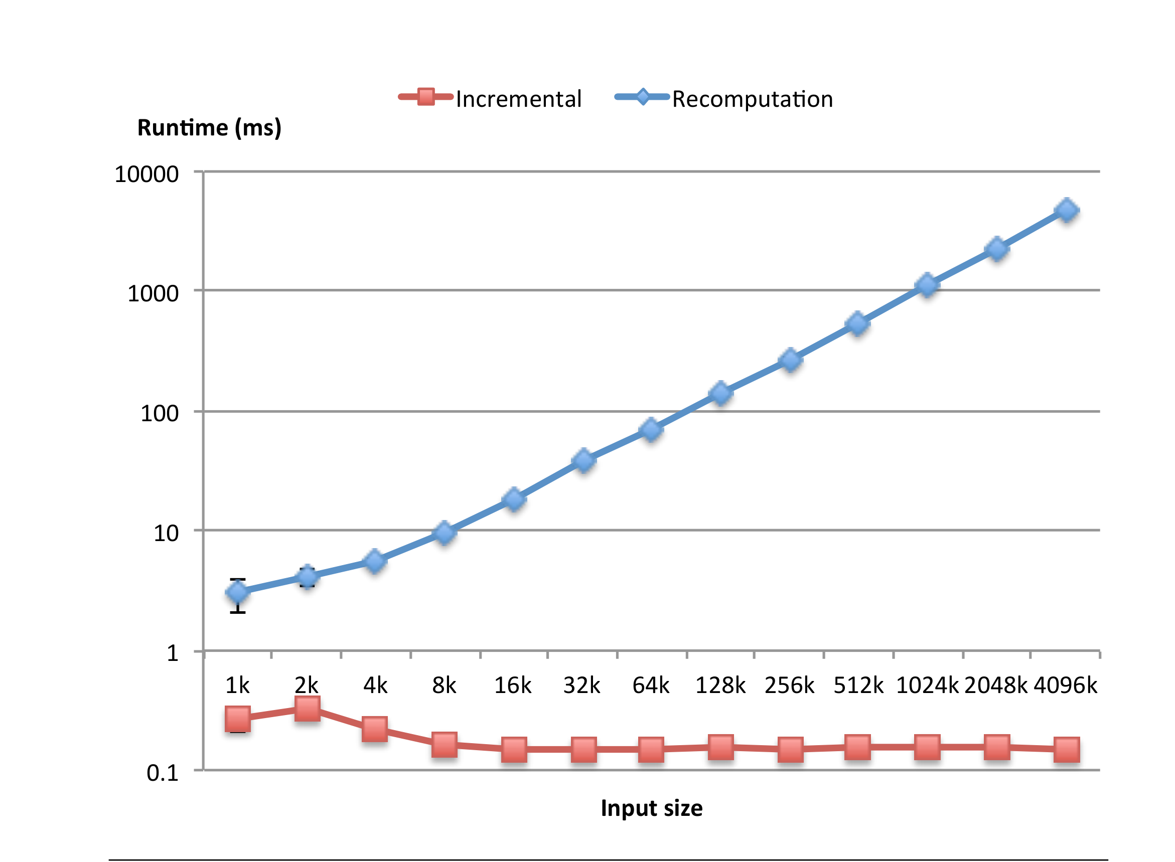
Our results show (Fig. 7) that our program reacts to input changes in essentially constant time, as expected, hence orders of magnitude faster than recomputation.

我们的结果（图 7）表明，我们的程序对输入变化的反应基本上是常数时间，这与预期相符，因此比重新计算快若干个数量级。常数因子足够小，因此在现实的输入规模上，加速比是明显的。

Constant factors are small enough that the speedup is apparent on realistic input sizes.

由于篇幅所限，关于基准测试结果与输入的细节可以在我们论文的扩展版（附录 A）中获得。

For lack of space, details on benchmarking results and inputs are available in the extended version of our paper (Appendix A).153 0.1 10000 Runme (ms) Input size Incremental Recomputa:onFigure 7.

图 7：性能结果（对数-对数坐标），横轴为输入规模，纵轴为运行时间（ms）。置信区间由误差条（whiskers）表示；大多数误差条太小而不可见。（原图见 PDF 第 10 页）

Performance results in log-log scale, with input size on the x-axis and runtime in ms on the y-axis.

从这些评估中可以得到两个重要的教训：

Confidence intervals are shown by the whiskers; most whiskers are too small to be visible. Two important lessons from the evaluations are: • As anticipated in Sec. 4.3, to achieve good performance our current implementation requires some form of dead code elimination, such as laziness. • Incrementalization increases code size significantly.

正如 §4.3 所预料的，要获得良好性能，我们当前的实现需要某种形式的死代码消除（dead code elimination），例如惰性求值（laziness）。

Analyzing and addressing this increase is left for future work.

增量化会显著增大代码体积。分析并应对这一增长留待未来工作。

5 相关工作5. Related work

Existing work on incremental computation can be divided into two groups: Static incrementalization and dynamic incrementalization. Static approaches analyze a program statically and generate an incremental version of it.

已有的增量计算工作可以分为两组：静态增量化与动态增量化。静态方法静态地分析程序并生成它的一个增量版本。动态方法在程序运行时建立动态依赖图，并沿这些图传播变化。

The trade-off between the two is that static approaches have the potential to be faster because no dependency tracking at runtime is needed, whereas dynamic approaches can support more expressive programming languages. ILC is a static approach, but compared to the other static approaches it supports more expressive languages. In the remainder of this section, we analyze the relation to the most closely related prior works. Ramalingam and Reps [21], Gupta and Mumick [13] and Acar et al. [3] discuss further related work.

两者之间的权衡在于：静态方法有潜力更快，因为运行时不需要依赖跟踪；而动态方法能够支持表达能力更强的编程语言。ILC 是一种静态方法，但与其他静态方法相比，它支持表达能力更强的语言。在本节余下部分，我们分析与最密切相关的前人工作的关系。Ramalingam 与 Reps [21]、Gupta 与 Mumick [13] 以及 Acar 等 [3] 讨论了更多的相关工作。

5.1 动态方法5.1 Dynamic approaches

One of the most advanced dynamic approach to incrementalization is self-adjusting computation, which has been applied to Standard ML and large subsets of C [2, 14]. In this approach, programs execute on the original input in an enhanced runtime environment that tracks the dependencies between values in a dynamic dependence graph [3]; intermediate results are memoized. Later, changes to the input propagate through dependency graphs from changed inputs to results, updating both intermediate and final results; this processing is often more efficient than recomputation.

最先进的动态增量化方法之一是自调整计算（self-adjusting computation），它已被应用于 Standard ML 以及 C 的大部分子集 [2, 14]。在这种方法中，程序在增强的运行时环境中对原始输入执行，该环境在动态依赖图（dynamic dependence graph）[3] 中跟踪值之间的依赖关系；中间结果被记忆化。随后，对输入的变化沿依赖图从被改变的输入传播到结果，更新中间结果与最终结果；这一处理通常比重新计算更高效。

However, creating dynamic dependence graphs imposes a large constant-factor overhead during runtime, ranging from 2 to 30 in reported experiments [4, 5], and affecting the initial run of the program on its base input. Acar et al. [5] show how to support high-level data types in the context of self-adjusting computation; however, the approach still requires expensive runtime bookkeeping during the initial run. Our approach, like other static ones, uses a standard runtime environment and has no overhead during base computation, but may be less efficient when processing changes. This pays off if the initial input is big compared to its changes.

然而，建立动态依赖图会在运行时带来很大的常数因子开销，在已报告的实验中为 2 到 30 倍 [4, 5]，并且会影响程序在其基础输入上的首次运行。Acar 等 [5] 展示了如何在自调整计算的背景下支持高层数据类型；然而，该方法在首次运行期间仍然需要昂贵的运行时簿记（bookkeeping）。我们的方法与其他静态方法一样，使用标准的运行时环境，在基础计算期间没有开销，但在处理变化时可能效率较低。当初始输入相对于其变化很大时，这样做是划算的。

Chen et al. [9] have developed a static transformation for purely functional programs, but this transformation just provides a superior interface to use the runtime support with less boilerplate, and does not reduce this performance overhead. Hence, it is still a dynamic approach, unlike the transformation this work presents. Another property of self-adjusting computation is that incrementalization is only efficient if the program has a suitable computation structure. For instance, a program folding the elements of a bag with a left or right fold will not have efficient incremental behavior; instead, it’s necessary that the fold be shaped like a balanced tree.

Chen 等 [9] 为纯函数式程序开发了一种静态变换，但这种变换只是提供了一个更好的接口，以便用更少的样板代码使用运行时支持，并没有降低这一性能开销。因此，它仍然是一种动态方法，不同于本文提出的变换。

In general, incremental computations become efficient only if they are stable [1]. Hence one may need to massage the program to make it efficient. Our methodology is different: Since we do not aim to incrementalize arbitrary programs written in standard programming languages, we can select primitives that have efficient derivatives and thereby require the programmer to use them.

自调整计算的另一个性质是：只有当程序具有合适的计算结构时，增量化才是高效的。例如，用左折叠或右折叠对多重集（bag）的元素做折叠的程序不会有高效的增量行为；相反，折叠必须呈平衡树的形状。一般来说，只有当增量计算是稳定的（stable）[1] 时，它才会变得高效。因此，可能需要改造（massage）程序以使其高效。我们的方法论不同：由于我们并不打算增量化用标准编程语言编写的任意程序，我们可以选择具有高效导数的原语，从而要求程序员使用它们。

Functional reactive programming [10] can also be seen as a dynamic approach to incremental computation; recent work by Maier and Odersky [18] has focused on speeding up reactions to input changes by making them incremental on collections. Willis et al. [24] use dynamic techniques to incrementalize JQL queries.

函数式响应式编程（functional reactive programming）[10] 也可以被看作一种动态的增量计算方法；Maier 与 Odersky 的近期工作 [18] 致力于通过让集合上的操作增量化，来加快对输入变化的反应。Willis 等 [24] 使用动态技术来增量化 JQL 查询。

5.2 静态方法5.2 Static approaches

Static approaches analyze a program at compile-time and produce an incremental version that efficiently updates the output of the original program according to changing inputs.

静态方法在编译期分析程序，并产生一个增量版本，该版本根据不断变化的输入高效地更新原程序的输出。

Static approaches have the potential to be more efficient than dynamic approaches, because no bookkeeping at runtime is required. Also, the computed incremental versions can often be optimized using standard compiler techniques such as constant folding or inlining.

静态方法有潜力比动态方法更高效，因为运行时不需要簿记。此外，计算出的增量版本通常可以用标准编译技术（例如常量折叠或内联）来优化。然而，它们都不支持一等函数；有些方法还有进一步的限制。

However, none of them support first-class functions; some approaches have further restrictions.

我们的目标是把静态增量化应用于表达能力更强的语言；特别地，ILC 支持一等函数，以及一个开放的、带有关联原语操作的基本类型集合。

5.2.1 有限差分5.2.1 Finite differencing

Paige and Koenig [20] present derivatives for a first-order language with a fixed set of primitives. Blakeley et al. [8] apply these ideas to a class of relational queries. The database community extended this work to queries on relational data, such as in algebraic differencing [13], which inspired our work and terminology. However, most of this work does not apply to nested collections or algebraic data types, but only to relational (flat) data, and no previous approach handles first-class functions.

Paige 与 Koenig [20] 给出了一个带固定原语集合的一阶语言的导数。Blakeley 等 [8] 把这些思想应用于一类关系查询。数据库社区把这项工作扩展到了关系数据上的查询，例如代数差分（algebraic differencing）[13]，它启发了我们的工作与术语。然而，这些工作大多不适用于嵌套集合或代数数据类型，而只适用于关系（扁平）数据，并且此前没有任何方法能处理一等函数。增量支持通常是针对整个语言整体地（monolithically）设计的，而不是逐块地（piecewise）设计的。改进了代数差分，Koch [15] 通过一种可组合的查询变换保证了渐近加速，并在现实的基准测试中带来了巨大的加速，不过仍然针对一阶数据库语言。

Incremental support is typically designed monolithically for a whole language, rather than piecewise. Improving on algebraic differencing, Koch [15] guarantees asymptotic speedups with a compositional query transformation and delivers huge speedup in realistic benchmarks, though still for a first-order database language. More general (non-relational) data types are considered in the work by Gluche et al. [12]; our support for bags and the use of groups is inspired by their work, but their architecture is still rather restrictive: they lack support for function changes and restrict incrementalization to self-maintainable views, without hinting at a possible solution.

Gluche 等 [12] 的工作考虑了更一般（非关系）的数据类型；我们对多重集（bag）的支持以及对群的使用受到了他们工作的启发，但他们的架构仍然相当受限：他们缺少对函数变化的支持，并把增量化限制在自维护视图（self-maintainable views）上，且没有暗示任何可能的解决方案。

5.2.2 静态记忆化5.2.2 Static memoization

Liu’s work [17] allows to incrementalize a first-order base program f (xold) to compute f (xnew), knowing how xnew is related to xold. To this end, they transform f (xnew) into an incremental program154 which reuses the intermediate results produced while computing f (xold), the base program. To this end, (i) first the base program is transformed to save all its intermediate results, then (ii) the incremental program is transformed to reuse those intermediate results, and finally (iii) intermediate results which are not needed are pruned from the base program. However, to reuse intermediate results, the incremental program must often be rearranged, using some form of equational reasoning, into some equivalent program where partial results appear literally.

Liu 的工作 [17] 允许增量化一个一阶基础程序 $f(x_{\mathrm{old}})$，在已知 $x_{\mathrm{new}}$ 与 $x_{\mathrm{old}}$ 之间关系的情况下计算 $f(x_{\mathrm{new}})$。为此，他们把 $f(x_{\mathrm{new}})$ 变换为一个增量程序，该程序复用计算基础程序 $f(x_{\mathrm{old}})$ 时产生的中间结果。为此，(i) 首先把基础程序变换为保存它的所有中间结果，然后 (ii) 把增量程序变换为复用这些中间结果，最后 (iii) 从基础程序中剪除不需要的中间结果。然而，为了复用中间结果，增量程序常常必须用某种等式推理（equational reasoning）重排为一个等价程序，使部分结果字面上出现。例如，如果基础程序 $f$ 使用左折叠对整数列表 $x_{\mathrm{old}}$ 的元素求和、从表头开始访问它们，而 $x_{\mathrm{new}}$ 在列表前面添加一个新元素 $h$，那么 $f(x_{\mathrm{new}})$ 在任何时刻都不会重新计算出相同的结果。但由于加法在整数上是可交换的，我们可以把 $f(x_{\mathrm{new}})$ 重写为 $f(x_{\mathrm{old}}) + h$。作者的 CACHET 系统会尝试自动进行这类重写，但不保证成功。类似地，CACHET 会尝试合成任何能由基础程序廉价计算出的额外结果，以帮助增量程序变得更高效。

Then, the differentiation algorithm computes incremental versions of user programs without requiring further user intervention. It would be useful to combine ILC with some form of static caching to make the computation of derivatives which are not self-maintainable more efficient. We plan to do so in future work.

由于很难完全自动化这类推理，我们把等式推理移到插件设计阶段。插件提供通用的高阶原语，插件作者已经为这些原语设计了高效的导数（在设计阶段使用等式推理）。然后，微分算法计算用户程序的增量版本，而不需要用户进一步干预。把 ILC 与某种形式的静态缓存结合起来，以使那些非自维护的导数的计算更高效，将会是有用的。我们计划在未来工作中这样做。

6 结论与未来工作6. Conclusions and future work

We have presented ILC, an approach to lifting incremental computations on first-order programs to incremental computations on higher-order programs. We have presented a machine-checked correctness proof of a formalization of ILC and an initial experimental evaluation in the form of an implementation, a sample plugin for maps and bags, and a non-trivial example that was incrementalized successfully and efficiently.

我们提出了 ILC，一种把一阶程序上的增量计算提升到高阶程序上的增量计算的方法。我们给出了针对 ILC 的一个形式化的、经过机器检验（machine-checked）的正确性证明，以及一项初步的实验评估，其形式包括一个实现、一个针对映射（maps）与多重集（bags）的示例插件，以及一个被成功且高效地增量化的非平凡例子。

Our work opens several avenues of future work. Our current implementation is not efficient on derivatives that are not selfmaintainable. However, as discussed (Sec. 4.3), we will study how to memoize intermediate results to address this limitation.

我们的工作开辟了若干未来工作方向。我们当前的实现在非自维护（non-self-maintainable）的导数上效率不高。然而，正如 §4.3 所讨论的，我们将研究如何对中间结果进行记忆化，以解决这一局限。我们的下一步将是开发具有高效非自维护原语的语言插件。

Our next step will be to develop language plugins which have efficient nonself-maintainable primitives. Another area of future work is adding support for algebraic data types (including recursive types), polymorphism, subtyping, general recursion and other collection types. While support for algebraic data types could subsume support for specific collections, many collections have additional algebraic properties that enable faster incrementalization (like bags). Even lists (which have fewer algebraic properties) can benefit from special support [18].

未来工作的另一个方向是增加对代数数据类型（包括递归类型）、多态、子类型（subtyping）、一般递归以及其他集合类型的支持。虽然对代数数据类型的支持可以涵盖对特定集合的支持，但许多集合具有额外的代数性质，能够实现更快的增量化（例如多重集（bag））。即使是（代数性质较少的）列表，也能从专门的支持中受益 [18]。

Moreover, we intend to apply ILC to optimize queries on collections in the context of the SQUOPT project [11], which was a motivation for this work; in particular, SQUOPT can automatically rewrite queries to use database-style indexes, and ILC enables updating those indexes when input data changes.

此外，我们打算在 SQUOPT 项目 [11] 的背景下应用 ILC 来优化针对集合的查询，该项目也是本工作的一个动机；特别地，SQUOPT 能够自动把查询重写为使用数据库风格索引的形式，而 ILC 使得在输入数据发生变化时更新这些索引成为可能。

Finally, we intend to perform a full and thorough experimental evaluation to demonstrate that ILC can incrementalize large-scale practical programs.

最后，我们打算进行一项全面而彻底的实验评估，以证明 ILC 能够对大规模的实际程序进行增量化。

致谢Acknowledgments

We would like to thank Ingo Maier, Erik Ernst, Tiark Rompf, other ECOOP 2013 participants, Sebastian Erdweg, Christoph Koch and the PLDI ’14 anonymous reviewers for helpful discussions and/or comments on previous drafts. This work is supported by the European Research Council, grant #203099 “ScalPL”.

我们感谢 Ingo Maier、Erik Ernst、Tiark Rompf 及其他 ECOOP 2013 参会者、Sebastian Erdweg、Christoph Koch 以及 PLDI ’14 的匿名审稿人，感谢他们有益的讨论和/或对先前草稿的评论。本工作由欧洲研究理事会（European Research Council）资助，基金号为 #203099 “ScalPL”。

高阶语言的变化理论A Theory of Changes for Higher-Order Languages